|
Other RHESSI |
|
|
|
|
|
|
|
|
|
|
|
|
David Smith, dsmith@ssl.berkeley.edu
Version 1, 02/04/01
This document is intended to introduce all the issues surrounding HESSI spectroscopy, i.e. the process of converting raw HESSI data to a spectrum in photons/cm2/s/keV originally incident on the spacecraft. Most of this conversion will be done automatically by the data analysis software with few decisions required of the user. Nonetheless, it is good for anyone intending to interpret HESSI spectra to know what the spacecraft and software are doing behind the scenes, beneath the surface, and before you see your spectrum. And despite the best efforts of the software team, there will be times when residual instrumental effects appear in your data; therefore it is good to consider whether something unexpected in your results might actually be due to one of the phenomena discussed below. This document contains sections on
The HESSI detectors
| The detector electronics
| The HESSI data formats
| Other devices on the instrument related to spectroscopy
| The detector performance
| Phenomena that can complicate or degrade spectroscopy, and
| The phases of a spectroscopy analysis.
| |
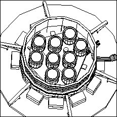
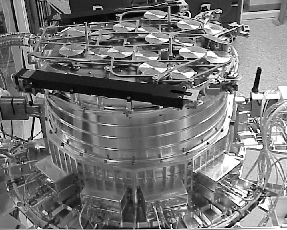
The arrangement of the HESSI detectors in the spectrometer (one beneath each grid) is shown in Figure 1. Figure 2 is a photograph of the assembled spectrometer before it was inserted into the bottom of the spacecraft. We refer to the detectors by the name of their grid pair: G1, G2, ... G9.
 |
 |
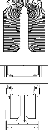 |
Each detector is a single crystal of hyperpure germanium in the general shape of a cylinder with a bore partway up the middle (see Figure 3). When hyperpure germanium is at cryogenic temperatures, no electron-hole pairs are in the conduction band, but a hard x-ray or gamma ray interacting in the crystal will release one or more energetic electrons, which lose energy by creating many free electron/hole pairs. If there is a high electric field (on the order of 1000 V/cm) across the crystal, the electrons and holes will be pulled to the electrodes, creating a current pulse. The total charge in the current pulse is proportionate to the photon energy.
Two conductive layers are implanted on the crystal surfaces to serve as electrodes: a thin, p-type layer of implanted boron on the front and side surfaces, and a thicker, n-type layer of diffused lithium ions on the inner bore. The rear surface is left as an insulator. The material overall is very slightly n-type, and when 2000-4000V is applied between the inner and outer electrodes the crystal is depleted of these charge carriers, with enough electric field in the crystal from the space charge and external voltage to cause the electron-hole pairs to reach terminal velocity. Most of the HESSI detectors will be operated at a high voltage (HV) of 4000V.
The step seen near the top of the inner bore in Figure 3 (top) is a break in the lithium contact. The signals are extracted separately from the two halves of this electrode. The line extending from this step to the outside edge of the detector represents a boundary electric field line: photons stopping above this line are detected in the front channel, and those stopping below it in the rear channel. Thus a single crystal becomes a stacked pair of detectors. The front segment will absorb all the hard x-rays up to about 100 keV, letting most gamma-ray line photons through. The rear segment will stop many of the latter, so that gamma spectroscopy can be done without high deadtime from the x-rays.
You may also hear the front segment referred to as the ``hemisphere'' or ``cap'' segment, and the rear segment referred to as the ``coax'' segment. We try to use the words ``segment'' and ``detector'' consistently: HESSI has 9 detectors and 18 segments.
The notch on the outer edge of the detector serves two purposes. First, it concentrates the electric field lines at the corner of the notch, so that the field line which originates at the inner step always hits the proper place on the outside of the detector. In addition, it removes some mass from in front of the rear segment, so that fewer high-energy gamma rays Compton scatter before entering the rear. To keep the ``shoulder'' part of the rear segment from being swamped with flare hard x-rays, a ring of thin ``graded-Z'' passive shielding is placed above the shoulder (Figure 3, bottom). This shield is just as effective as the front segment in photoelectrically absorbing hard x-rays, but with much less Compton scattering of gamma-rays. The graded-Z shielding consists of 0.5mm of Ta, 1mm of Sn, 0.5mm of steel, and the aluminum which is part of the cryostat structure. Each element stops the K-shell fluorescence photon from the higher-Z element before it. The whole is opaque up to about 100 keV. Additional graded-Z shielding is put in a ring around the edge of the front segment to stop background photons from the Earth and cosmic diffuse background, and on top of the spectrometer in the area between detectors to stop x-rays from scattering around in the spectrometer and entering the rear segments from the side.
The HESSI electronics produce a series of photon events (4 bytes each) containing the energy, time, and detector segment of the photon plus some encoded livetime information. There are two other data formats produced as well: ``monitor rates'', which are 1-second accumulations of various counters related to activity in the detectors (see below), and, at times of very high count rate, ``fast rates'', which record the count rate in each segment at a very fast cadence (also see below).
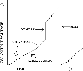 |
The first stage of amplification comes in an FET immediately behind the detector. The signal from the FET is taken by a special low-thermal-conductivity harness out to the rest of the Charge Sensitive Amplifier (CSA). One CSA for each detector sits along a ring around the outside of the spectrometer, alongside the HV filter which conditions the HV for the same detector. The CSA amplifies the signal further and also drives a reset transistor for each segment (which is located next to the signal FET inside). The reset transistor drains the accumulated charge whenever the total accumulated energy from photon interactions, particle interactions, and leakage current for its segment is about 40 MeV. Figure 4 shows, schematically, the raw output of the CSA.
You may also hear the CSA referred to as the ``preamp''.
The CSA signals for front and rear segments are sent to a Detector
Interface Board (DIB). There is one DIB for each detector, and
they are located in the Instrument Data Processing Unit (IDPU) box.
The signal chain for each of the 18 segments is split into two:
a fast chain which converts each event (step in the raw CSA
signal) to a pulse of about 800 ns total width, and a slow chain
which converts each event into a pulse of about 12 ![]() s total width.
The slow signal, which has very good energy resolution because of
the long integration time, is sent to the analog-to-digital
converter (A2D) to produce the pulse heights written into each event.
The fast pulse has poorer energy resolution but is used for
decisions which have to be made quickly, i.e. pileup rejection and
gain switching (see below), and for generating fast rate data
when counting rates are too high to do event-by-event spectroscopy
(also see below).
s total width.
The slow signal, which has very good energy resolution because of
the long integration time, is sent to the analog-to-digital
converter (A2D) to produce the pulse heights written into each event.
The fast pulse has poorer energy resolution but is used for
decisions which have to be made quickly, i.e. pileup rejection and
gain switching (see below), and for generating fast rate data
when counting rates are too high to do event-by-event spectroscopy
(also see below).
Both the fast and slow channels have lower-level discriminators (LLDs). For the front segment, these are set as low as possible without triggering on random noise: about 3 keV for the slow channel and 6 keV for the fast channel. One front segment (G7) has these thresholds set a little more than a factor of 2 higher due to an extra white noise source in that channel. For the front segment, the slow LLD must trigger to signal the A2D to begin digitizing and produce an event. For the rear, both thresholds must be exceeded for the A2D to produce an event, and both are set near 20 keV. Below 20 keV, photons approaching the rear segment from any direction will be stopped by passive material or by the front segment.
The A2D produces a 13-bit (8192 channel) pulse height value for each event. Gain is extremely linear, with deviations of < 1 keV from linearity across the whole scale. The approximate gain function for the front segments is Energy(keV) = Channel*0.35 - 12 keV, giving an energy range up to about 2.8 MeV. Note that this places zero energy around channel 34. There are significant variations from segment to segment, but variations with time, temperature, etc. for any one segment should be small (<<1%). Nonetheless, because the resolution is so high, we anticipate keeping a database of gain variations with time in order to get the best possible performance from the detectors. These gains will be calculated orbit-by-orbit from fitting the positions of background lines. The spectroscopy tools will select the appropriate gain function in a way that should be invisible to the user.
 |
The rear segments have a gain function near Energy(keV) = Channel*0.39 - 12 keV, or up to about 3.2 MeV. To analyze gamma-rays at even higher energies, there is a second gain range added to the rear segments. The pulse from the fast chain is sent out ahead of the slow spectroscopy signal. If its amplitude is higher than a certain threshold (about 2.9 MeV), the gain of the A2D is changed so that the 8192 channels represent an energy scale about a factor of 5.2 higher (to 17 MeV). There is a bit in the 4-byte rear-segment event to tell which gain level the 13-bit channel value was taken with. Because the resolution of the fast signal is poor, the transition from one gain level to another is not abrupt: i.e, photons in the range 2.6-3.2 MeV can appear at either gain. By using events from both gain ranges, however, an undistorted spectrum can be reproduced. Figure 5 shows how data taken with a high-energy source (56Co) are split between the two gain ranges. Most of the time, the spectroscopy tools will automatically search both gain ranges for events if the user has asked for data in the 2.6-3.2 MeV range.
If there are two events less than 800ns apart, their energies will
be added together (piled up) - this is unavoidable, but should
happen very seldom except in the largest flares. For event separations
of 800ns to 6![]() s, the DIB will veto both events based on the two
fast signals, since the slow signals would overlap and contaminate
each other, distorting the energy value. For event separations from
6 to 9
s, the DIB will veto both events based on the two
fast signals, since the slow signals would overlap and contaminate
each other, distorting the energy value. For event separations from
6 to 9 ![]() s, only the second event would have its energy distorted,
so only the second event is vetoed. In the front segment, events
below about 6 keV (which don't trigger the fast LLD) can pile up
unrestrictedly on other events. The pileup correction code will
take this into account.
s, only the second event would have its energy distorted,
so only the second event is vetoed. In the front segment, events
below about 6 keV (which don't trigger the fast LLD) can pile up
unrestrictedly on other events. The pileup correction code will
take this into account.
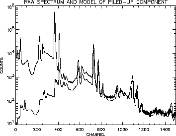 |
Pileup correction is an iterative process which is based on the shape of the raw spectrum and knowledge of the count rate and measured livetime. After the spectral shape is corrected to first order (see Figure 6), the corrected spectrum can be fed back into the algorithm for successively finer corrections. For the majority of flares, pileup correction will be unnecessary, and for the majority of the remainder, the first-order correction will suffice.
Livetime, on the other hand, is independent of the energy, and the livetime correction changes only the overall magnitude of the spectrum (i.e. photometry) rather than the spectral shape. The livetime of a detector is simply the probability that one additional photon, put in at a random time, would in fact be recorded. Deadtime is (1. - livetime), the percent time that the circuit is ``tied up'' by other events. The livetime signal for each segment is a logic line which is ``OR''-ed together from several lines in the circuit, representing several reasons the circuit could be unable to process an event (A2D in use, pileup rejection active, CSA reset in progress, etc.) This line is sampled at 1 MHz and the livetime reported in the monitor rates is the fraction of these sample strobes which read the line as clear.
Because the pileup circuit can sometimes choose to veto BOTH events rather than just one, there is a loss of livetime due to pileup rejection which cannot be measured just by sampling the pileup-rejection logic line. Therefore the livetime correction routines do not use the ``raw'' livetime measurement as reported in the monitor rates, but a corrected livetime which is somewhat lower.
The maximum event throughput is about 25,000-30,000 counts per segment per second and it is reached at about 50% livetime.
Most of the time, whether a flare is active or not, every photon event in the HESSI detectors is stored in onboard memory as 4 bytes of data and telemetered to the Berkeley ground station (or a backup station) within a day or two. Each event contains:
5 bits identifying the segment and (if a rear
segment) energy range of the event,
| 13 for the energy channel,
| the last 10 bits of the time counter, giving the
event time in units of binary microseconds (i.e. 2-20 seconds), and
| 4 bits which are a partial measurement of the livetime counter.
The livetime counter is read every 1/2048 second and its 9-bit value is
broken up into 3-bit chunks and placed in this data slot in three
consecutive events from that segment. The 4th bit is set to 1 to
indicate where this
sequence of three events begins. If the events are not coming
quickly enough to produce a continuous livetime readout this way,
they still produce a sampling of it.
| |
If the onboard memory starts to fill up, a decimation algorithm automatically throws out all but one out of every N events in the front segments below a certain energy E, with N from 2-16. E and N are functions of both the remaining memory and the position of the attenuators (see below). Decimation in the rear segments can be commanded as a routine way of keeping background (mostly photons from the Earth's atmosphere or the cosmic diffuse background) from filling up the memory. For example, a high level of decimation can be commanded for times when HESSI is in shadow.
Monitor rates are a separate kind of data packet (``AppID'' in telemetry parlance) produced once every ten seconds. Each packet consists of 10 1-second accumulations of a set of counters for each of the 18 segments. The counters are: number of resets, number of slow LLD triggers, number of fast LLD triggers, number of upper-level discriminator (ULD) triggers on the slow channel (i.e. events above the energy of channel 8192 - usually cosmic rays), and fraction of ``live'' results from the livetime strobe. This information is normally used to check the health of the detectors and is not necessary for spectroscopy.
Due to an oscillation in the CSA that occurs only during a reset, the reset counters in the rear segments increment multiple times on each actual reset; the multiplicity factor for each segment is known and will be available to any software that uses these data.
Fast rates are yet another data format, produced only when the count rates are very high. The data are count rates in four broad energy bands (all in the hard x-ray range). The pulses are sampled from the fast electronics chain. The rates for the three detectors (1,2,3) with the finest grids (and therefore fastest imaging modulations) are sampled at 16 kHz; the next three (4,5,6) at 4 kHz; and the three coarsest grids (7,8,9) at 1 kHz. Events are not shut off when the fast rate data turn on; however, at these very high count rates the event data will naturally taper off due to very high deadtime.
There are two attenuators designed to cut down the photon flux during bright flares so that the detector deadtime stays below 50%. Each attenuator is a set of 9 aluminum disks held in a lightweight frame. Each frame has only two positions: one with the disks covering the detectors and one with the detector field of view completely clear. They are moved automatically in response to increases and decreases in the monitor rate counters. The frames are moved by putting a high current through shape-memory alloy (SMA) wires which then contract. The move takes less than 1 second, so there will be only a short time when the instrument response is in transition between well-calibrated states.
Each attenuator disk consists of three concentric regions of differing thickness. The ``heavy'' disks have a thick outer region covering most of the detector area, a thin middle region of smaller area, and a tiny, very thin spot in the center. The ``light'' disks have only thin aluminum in the large outer area, thick aluminum in the middle region, and a very thin spot in the middle somewhat larger than that of the heavy disk. Together, these disks provide four levels of attenuation which allow HESSI to have an enormous dynamic range of sensitivity and make useful measurements over 6 orders of magnitude in incident flare (or microflare) flux. When the attenuators are both in place, there is thick aluminum over both the outer and middle regions, and only the smallest spot in the very center admits the soft photons which are so prolific in the thermal (post-impulsive) phase of large flares.
You may also hear the attenuators referred to as ``filters'' or ``shutters''.
For the first few months of HESSI's operation, the light attenuator will be locked over the detectors and the heavy attenuator locked out of the way. After that, the attenuators will be free to move based on an algorithm which attempts to keep the deadtime below 50% while including some hysteresis to avoid having the attenuators ``chatter'' in and out during periods when the flux is near a threshold.
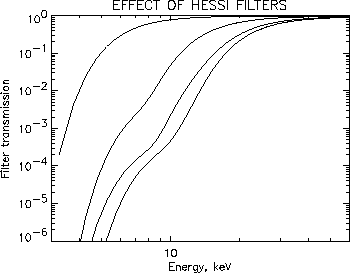
Figure 7 shows the attenuation caused by the thermal blankets and beryllium windows above the detectors (top trace) and the attenuation with the thin, thick, and combined attenuators.
HESSI carries a tiny onboard radioactive source (5 nanocuries of 137Cs) which makes a line at 662 keV, far from any line expected to occur in flares or in HESSI's variable background. The count rate from this source is so small that it can only be detected in spectra accumulated over many hours. The line of known intensity lets us monitor any changes in the efficiency of the detectors such as might occur via radiation damage (see below). The same function can be served by a line at 1460 keV from naturally occurring 40K in the spacecraft, but the absolute flux of this line is not known before launch since there is always some of the isotope in the laboratory. Other sources of background will be far more important in determining the sensitivity of HESSI.
Since the rear segments see no direct flare photons below 100 keV, we can use them at these low energies as a crude hard x-ray polarimeter. There is a cylinder of beryllium 3 cm in diameter and 3.5 cm long nestled among the rear segments (see Figure 1). Above this cylinder is a thin spot in the spectrometer shell and a hole in the grid trays, so that solar photons > 20 keV can reach the cylinder and scatter into the adjacent rear segments. The Klein-Nishina cross section, differential in azimuth angle, is a function of the angle from the polarization axis. Thus, by watching the relative rates of these rear segments, we will measure the direction and degree of polarization for incoming photons of roughly 20-100 keV. Simulations suggest that we will be able to detect polarization fractions as low as a few percent for the largest flares. The key difficulty in the analysis will be photons scattered from the Earth's atmosphere, which also produce low-energy counts in the rears and which also vary with the spacecraft spin.
The IDPU can put regular, small pulses into the detectors' HV supply, which the electronics see as equivalent to photon events. The pulse energy can be tuned across the detectors' full range, but the front/rear ratio is fixed at roughly 1:3 because the HV is shared by both segments and their response is proportional to their capacitance. Pulse rates can be commanded separately for each detector at 11 discrete frequencies, spaced by a factor of two, up to 1024 Hz. This pulser is not required in flight, but may be used for diagnostics.
 |
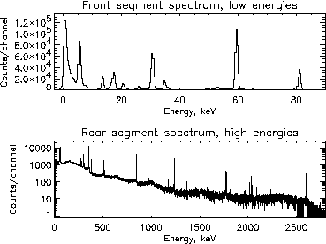 |
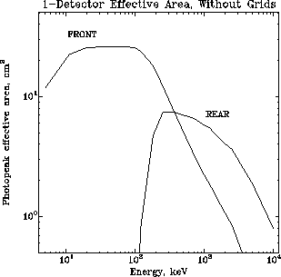
The effective areas of single HESSI front and rear segments are shown in Figure 8, from a simulation with an accuracy of a few percent. Figure 9 shows front and rear spectra from a typical HESSI detector. The energy resolutions (FWHM) are about 920 eV in the front and 2.75 keV in the rear. The 5.9 keV line from 55Fe can be seen in the front-segment spectrum. The noise counts below it (at about 1-3 keV) are false ``image events'' (see below) related to true events in the rear segment. They can be removed by the data analysis software without affecting real 3 keV events.
The effective area, resolution, and predicted background level allow us to calculate HESSI's sensitivity to the gamma-ray lines in flares. Even though HESSI carries no shielding to block background photons from the Earth or the cosmic diffuse sky, the flares which will show gamma-ray lines are so intense that the bremsstrahlung emission from the flare itself will overwhelm these sources of background, and will therefore define the continuum above which the lines must be detected.
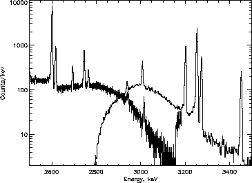
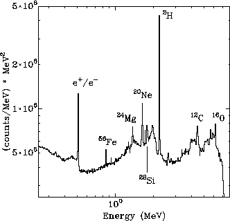
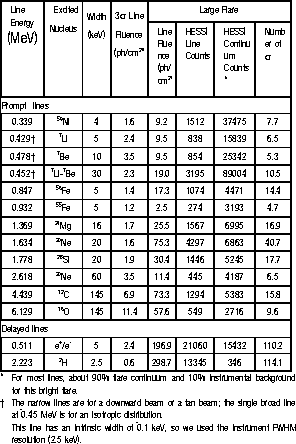
Figure 10 shows the expected HESSI response to a intense
gamma-ray line flare, with the origin of many of the lines
labeled. Figure 11 shows the expected sensitivity to these and other
lines, defined in two ways: the statistical significance of
each line for the largest expected gamma-ray line flare, and the
line flux required for a 3![]() detection.
detection.
When the clouds of electrons and holes liberated by a gamma-ray event move through the detector, they create induced charges on the electrodes of the segment in which they are moving. The change in time of this induced charge actually creates the current pulse which is amplified and integrated by the CSA to become the detected event. However, they also induce charges on the electrodes of the empty segment. The difference is that the image charges reverse sign in the empty segment as the clouds approach the electrodes of the segment in which they are actually moving. The result is that the image signals (current vs. time) in the empty segment are bipolar in shape and integrate to zero charge.
 |
The HESSI electronics, however, do not integrate the signals for an infinite time; the peaking time of the shapers is only a few microseconds. Therefore a small amount at the very end of each pulse is not counted. Since it is the negative part of the bipolar signal in an empty segment that comes last, the result is that there is a very small, positive residual from the bipolar signal: in other words, a 1 MeV event detected in one segment will create a simultaneous (but false) event in the other segment of a few keV.
There are two other ways events can be coincident between two segments (or two detectors): there could be real energy deposits in both segments from the same initial photon or cosmic ray (we sometimes call this a ``true coincidence'') or there could be two separate photons that arrive nearly at the same time by chance (``accidental coincidence'').
Usually, the simplest way to do spectroscopy is to throw out all coincident events (defined as events within N binary microseconds of each other, where the best value of N is 4 or 5). When you want to get every last photon to detect a faint gamma-ray line, however, you will want to include front/rear coincidences and coincidences between adjacent rear segments (the software will have a single flag to specify this configuration). When the count rates are very high, you may not want to reject coincidences at all, since a large fraction of events will be accidental coincidences.
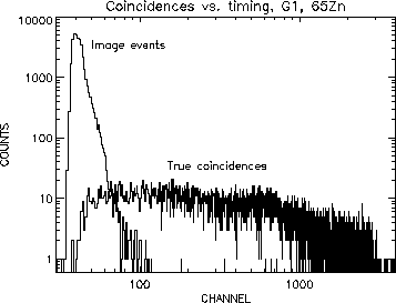
At moderate count rates, it is possible to separate image
events from true coincidences by the precise relative timing
of the two events. If the separation in binary microseconds
between the two events is ![]() ,
then this table describes
the relation between the events:
,
then this table describes
the relation between the events:
First EventEvents of any other spacing are probably accidental coincidences. Figure 12 shows how sorting coincident events byEvent type
FRONT 1 Image event in front
FRONT 0 Image event in front
REAR 0 True coincidence
REAR 1 True coincidence
REAR 2 True coincidence
REAR 3 Image event in rear
REAR 4 Image event in rear
You may also hear image events referred to as ``bipolar pulses'' or ``false coincidences''.
Radiation damage has always been a major performance issue for germanium detectors in space. Nuclear interactions with high-energy protons or neutrons cause displacements in the Ge crystal lattice. These displacements can become traps which remove some of the holes liberated by a gamma-ray interaction as they travel through the crystal. The electrons moving in the opposite direction from these holes are relatively immune. This trapping broadens a gamma-ray line in a way proportional to its energy, because gamma-ray interactions in some parts of the crystal force the holes to move through more damaged germanium than interactions in other parts, and thus different gamma-rays of the same energy suffer different percentage amounts of signal loss through trapping.
 |
HESSI's orbit grazes the inner edge of the proton belt a few times a day at the South Atlantic Anomaly (SAA). Most of the trapped protons (those below about 40 MeV) are stopped by the aluminum surrounding the detectors, but protons from 40-100 MeV interact in the outer few mm of the detector and the (relatively few) protons around 200 MeV and higher produce damage throughout the crystal. A smaller amount of damage throughout the crystal is caused by cosmic rays.
The damage is minimized in several ways. First, since the holes travel to the outer electrode and most of the detector volume is at large radii, most hole clouds travel only a short distance through damaged germanium. Second, we will keep the detectors very cold (70-80K), even though they can operate at much higher temperatures (up to 110K or higher), and keep the HV on at all times. Although the number of crystal displacements is only a function of the radiation dose, very low temperatures and uninterrupted HV can prevent the accumulated crystal displacements from becoming active as traps. Third, a few of the HESSI crystals have a scattering of naturally occurring electron traps due to impurities in the crystal. For these detectors, the resolution will actually become slightly better at first as hole traps are created: when electrons and holes are equally trapped, there is no effect on the line shape, just a slight overall decrease in gain. Fourth, for some minutes after HESSI emerges from the SAA, the large currents that were going through the detector while it was bathed in the radiation belts will have filled up all the traps in the crystal, so that the resolution will be temporarily better. Within one orbit, however, the traps will empty out again.
Finally, we have heaters near the detectors which can bring the array
to
![]() C; annealing for about a day at this temperature
should remove most of the accumulated radiation damage. From our
estimate of the proton dose on orbit, we expect to anneal after the
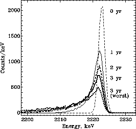
HESSI baseline mission of two years. Figure 13 shows the expected
profile for the 2.2 MeV line (neutron capture on ambient protons in
the solar atmosphere) as a function of elapsed mission time. Note
that only the two delayed lines from flares, 511 keV and 2.2 MeV, are
narrow enough for radiation damage to matter. All the other solar
lines are broad enough that their natural width is higher than any
amount of resolution loss we might expect from radiation damage.
C; annealing for about a day at this temperature
should remove most of the accumulated radiation damage. From our
estimate of the proton dose on orbit, we expect to anneal after the
HESSI baseline mission of two years. Figure 13 shows the expected
profile for the 2.2 MeV line (neutron capture on ambient protons in
the solar atmosphere) as a function of elapsed mission time. Note
that only the two delayed lines from flares, 511 keV and 2.2 MeV, are
narrow enough for radiation damage to matter. All the other solar
lines are broad enough that their natural width is higher than any
amount of resolution loss we might expect from radiation damage.
Detector G8 has a particularly high concentration of natural electron traps, particularly in the front segment. This produces poor resolution at high energies in this detector now, but it will improve as it accumulates hole traps through radiation damage, and continue to improve while other detectors start to deteriorate.
The cryocooler that keeps the detectors cold is a Stirling-cycle refrigerator with a piston that operates near 58.6 Hz. It contains an actively-driven counterweight which moves opposite the piston to cancel out most of the vibration, but there is still vibration transmitted to the spacecraft at higher frequencies (harmonics of the piston frequency and even higher frequencies which may be related to valves or other moving parts in the cooler). Vibrations can cause a degradation in the resolution of the HESSI detectors by the same principle used in a capacitor microphone: small motions make small changes in capacitance, producing small changes in voltage, which are read as noise on the CSA output. The susceptible capacitance could be in any of several places in the detector/HV/FET system.
For the most part, the HESSI detectors are resistant to this sort of noise, through both mechanical design features and the design of the DIB electronics (baseline restorer circuit). Several of the detectors display a minor loss of resolution, however, mostly due to what we believe is a mechanical resonance with the 14th harmonic of the piston frequency (820 Hz). The severity of this problem varies with the cryocooler power and the temperature of the spectrometer shell (and therefore the cryocooler body). By adjusting the cooler power and by operating heaters on spectrometer exterior, we have shown that this problem can be kept minor.
The front segment of the detector G2 has a more severe and variable degradation of resolution when the cryocooler is on. We hope this will be sufficiently stable on orbit that we can maintain a database of its state that will allow the software to automatically account for this degradation when you do your analysis. However, whenever you are doing spectroscopy separately from imaging, it will be best to explicitly remove this detector from the analysis - it could be anywhere up to a factor of 5 worse in resolution than the other eight front segments.
Because the microphonics effects all occur at low frequencies compared to the risetime of a single photon pulse, they affect only the energy resolution: unlike the white noise source in the front segment of G7, they cannot produce false events at low energies and therefore do not affect the setting of the LLDs (and therefore the low-energy limit of our observations).
A very small fraction of events near or above 3 MeV that should be analyzed with the high-energy gain range of the rear segments do not trigger the gain shift in the fast channel, and therefore pile up in the top few (64) channels of the low-energy scale (see Figure 5). This should be the first interpretation for any unexpected excess around 3 MeV. To verify, look at the raw data (in channel space rather than energy space) and see that the extra counts correspond to the top 64 channels (8128-8191). We expect to have the data analysis software deal with this problem by looking only at the events tagged for the high-energy scale in making spectra for this energy range. The small number of counts piled up at the bottom of the low-energy range will be redistributed according to the spectral shape determined from the high-energy range in order to get the correct intensity in that band.
At extremely high rates only, a similar artifact appears in the 64 channels preceding the halfway point of the spectrum (i.e. channels 4032-4095). When analyzing the brightest flares, the user should remain aware what of energy range this channel range maps to and be cautious interpreting results there.
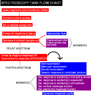
Figure 14 gives a schematic representation of the various steps involved in a spectral analysis. In general, you will be able to specify which steps listed here are done, and how they are done, by a few very simple operations. It is important that they be done in the order treated below, or the result will be wrong; we'll try to make it hard or impossible for you to take these steps in the wrong order. The default analysis which you will get if you take no special actions and set no flags will be a relatively simple one, optimized for hard x-ray flares of modest intensity.
Imaging spectroscopy is beyond the scope of this document. The modulation introduced by the grids does have some energy dependence. Therefore, to make sure that the modulation has no distorting effect on your spectrum, you should take spectra whose duration is an integral number of half spins whenever possible.
A general note: spectroscopy analyses will be more accurate when the whole procedure down to the last step is done separately for every segment. For example, imagine that one segment has a much higher livetime than another, and is also picking up a slightly different-shaped spectrum (more background, perhaps). If you do an averaged livetime correction to a spectrum which is the sum of these two segments, their relative contributions will be incorrect. Similarly, if the count rate varies dramatically during the period of your analysis, the time intervals of high and low livetime in EACH segment should also be analyzed separately. If you want a summed spectrum over a long time, you can analyze it in pieces and average together the results at the end. We will try to make this easy for you to do, but it will sometimes be easier, for a quick look, to sum events from many segments and time intervals together and do a single pass through the steps listed below considering the entire spectrometer (or a set of segments you've chosen) as the detector.
A spectrum can be produced from one or more segments, and with and without coincidence in various modes. In general, for work below 100 keV, you should choose just the front segments (usually minus G2). For higher energies, include the rear segments. For even higher energies (above the annihilation line at 511 keV), it will probably be useful to start including (true) coincident events between the front and rear segments and between adjacent rear segments. The spectroscopy software will treat each possible combination of two segments as a ``virtual segment'', with its own gain correction, efficiency, etc. Any use of coincident events at all is considered an advanced function, and may not be available in the software at launch.
The software will use the best possible gain data for each segment; either a best-guess single function for each segment, or, if available, one which includes the small variations with time.
The software can bin the data from all the segments (except the high-energy range of the rear segments) up to a standard finest binning of exactly 1/3 keV per bin, starting exactly at 0 keV, and going to 3 MeV in 9000 bins. This preserves just about all the information in the original spectra. The standard binning for the high-energy range is exactly 2 keV per bin.
It would be prohibitively difficult in terms of computer memory and processing time to try to do the spectroscopy analysis in this full set of bins, however, particularly if using the full response matrix (see ``Full Response Correction'' below). The spectrum would look pretty bad, too, since there would be few counts in each bin in most cases. Therefore you must choose your own binning, and you should choose a binning fine enough to accomplish the scientific goal but otherwise giving as small an array as possible.
On the other hand, if the bins are TOO broad, the response,
background, etc. will change too much across each of your bins for the
average value to be a good representation - this is analogous to the
perils, described above, of combining segments or time periods which
are very different. As a rule of thumb, you shouldn't expect good
results from bins with ![]() E > E/10.
E > E/10.
You will be able to specify binnings with different widths at different
energies. One example would be a logarithmic binning, where ![]() E/E
is nearly constant; another would be a binning that gets fine only around
narrow gamma-ray lines and is coarser everywhere else. We will provide
a selection of convenient binnings that you can choose just by referring
to a number, and these will probably be enough for most uses, although
you can always make up your own.
E/E
is nearly constant; another would be a binning that gets fine only around
narrow gamma-ray lines and is coarser everywhere else. We will provide
a selection of convenient binnings that you can choose just by referring
to a number, and these will probably be enough for most uses, although
you can always make up your own.
The currently available set of ``canned'' binnings is not complete, but such ones as we currently have will remain available with the same numeric codes as we add new ones. If you have an idea for a binning you think might be of general interest, please let me know. The binning files live in the ``dbase/spec_resp'' directory and have names of the form ``ct_edges.N'' where N is the identifying number. These are ASCII files; the first number in the file is the number of bin edges, which is one more than the number of bins. The rest of the numbers are the energy, in keV, of the bin edges. The currently available values of N correspond to these binnings:
0: Three energy bands, 10 keV wide, starting from 20 keV.
We use it mostly for quick software checks, but it
could be useful for some hard x-ray work.
|
1: 99 1-keV bands, covering 1-100 keV. Possibly good for
high-resolution hard-x-ray work (fitting
thermal and nonthermal emission, etc.)
|
2: The three bands from "0" plus 50-100 and 100-200 keV
bands; we will probably use this binning for a lot
of non-solar work with the rear segments.
|
3: A broad band from 20-200 keV followed by 6 narrow
bands (4 keV wide) to 224 keV. Used in software
debugging.
|
4: 1000 1-keV bands from 3-1003 keV. Mostly useful for
generating finely-detailed response matrices for
debugging and display purposes.
|
5: 565 bands: 1 keV each up to 100 keV, then 5 keV
bands to 1820 keV, and 10 keV to 2500. In addition,
there are sections of fine binning around the 511 keV
and 2.2 MeV lines. This is a good choice for first-look
spectroscopy of gamma-ray flares.
|
6: 199 bands: 1 keV binning 1-100 keV, then 5 keV binning
to 600 keV. A more complete binning than "1" for studying
hard x-ray continuum spectra out to higher energies.
|
7: 19 bands: 10-keV bands from 10-100 keV, then 50-keV
bands to 600 keV. Good for survey work to select
spectra for closer analysis with "6".
|
8: 78 bands: 3-keV bands from 1 to 118 keV, then 15-keV
bands up to 703 keV. Intermediate between "6" and "8"
in memory use for hard x-ray work.
|
9: 4 12-keV bands from 200-248 keV. Another debugging
mode.
|
10: 9 bands with pseudo-logarithmic binning covering the whole HESSI
energy range. The bin edges are at
[3, 6, 12, 25, 50, 100, 300, 1000, 2500, 20000] keV. These spectra
should contain all the events in the HESSI data stream (minus
any rejected by event selection criteria like segment
choices or coincidence rejection). Potentially useful for
quick screening to separate x-ray from gamma-ray flares,
etc.
| |
Livetime correction, as mentioned above, affects only the intensity and not the shape of a spectrum, although it can affect the shape indirectly if different livetime corrections are applied to different segments which recorded different spectra.
The pileup correction will be small for all but the largest flares, but we will try to have at least the first-order pileup correction available in time for launch.
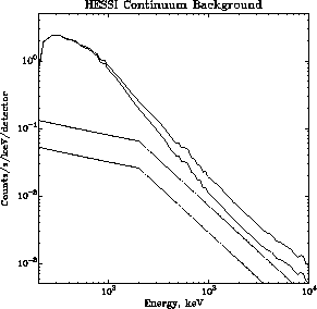 |
HESSI is an unshielded, high-background instrument like BATSE on CGRO or TGRS on Wind, not a shielded instrument like the Gamma-Ray Spectrometer on SMM was. Therefore it will be necessary to subtract background even in the case of bright flares. Our best estimate of the continuum background is shown in Figure 15. Below about 100 keV, the dominant source of background will be the cosmic diffuse hard x-ray background. Above 100 keV, the dominant source will be the hard x-ray and gamma-ray glow of the Earth's atmosphere resulting from cosmic-ray bombardment. There will also be gamma-ray lines from activation of the detectors and surrounding material by cosmic rays and by radiation-belt protons. Immediately after each passage through the South Atlantic Anomaly, this last component will be extremely bright.
The simplest way to estimate the background is to average spectra from just before and just after your flare; this will be the default, and the software will show you a lightcurve (count rate vs. time) and ask you to pick what time intervals you would like to use for background (and for your ``source'' or flare interval, too, of course).
Sometimes, however, a flare will last for the better part of an orbit, or occur just after sunrise or just before sunset, so that this technique won't give a good result. Eventually, there will be three other choices, which you should try in this order:
Background data taken from one orbit before and one orbit after
the flare, at the same orbital phase as the flare data.
| Background data taken from 15 orbits (1 day) before and 15 orbits after
the flare, at the same orbital phase as the flare data.
| Background generated by interpolation from a large database of many
background spectra, sorted by various parameters such as the
Sun-Earth-HESSI angle, magnetic latitude, time since last
SAA passage, etc.
| |
Needless to say, the last item will be quite a while in coming.
 |
There remains only to correct for the efficiency of the instrument (i.e. the loss of counts to absorption in passive material), and possibly for scattering (i.e. for the movement of counts from their original energy to some other energy). The former correction is much easier, since it involves only multiplying each bin of the spectrum by a correction factor. Once this is done, we no longer give the spectrum units of ``counts'', but rather of ``photons'' (or photons/cm2/s/keV, etc.).
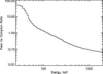
In many cases, it will only be necessary to do the efficiency correction. Below 100 keV, more photons leave all their energy in the detector than scatter and leave less energy. This is shown in Figure 16, which shows the ratio between the number of counts in the photopeak and the number at lower energy (in the ``Compton tail''). Below about 40 keV the Compton tail is truly negligible; but between 40 keV and 100 keV virtually all flare spectra fall, more or less steeply, so that even if the number of Compton tail counts from 100 keV photons is equal to the number of photopeak counts, it is dwarfed by the photopeak events from the lower energy photons. Thus, for hard x-ray work, the simple correction based only on the photopeak efficiency will give a spectral shape very close to the correct one.
For the study of narrow gamma-ray lines, only the photopeak efficiency is needed, since the user is not concerned with the shape or intensity of the continuum. This is certainly true for the very narrow lines at 2.2 MeV and 511 keV, but will also be a good approximation for the narrower excitation lines as well.
 |
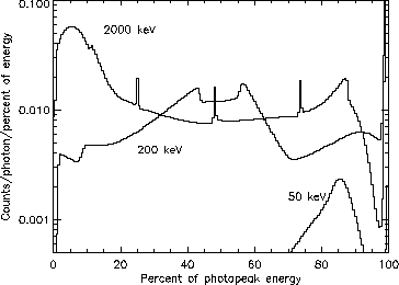
The full response matrix will have to be used when looking at the overall shape of the gamma-ray spectrum. Figure 17 shows the response of the instrument to incident photons of three energies: 50, 200, and 2000 keV. They are each scaled so that the photopeak energy is at the right edge of the plot. At 2000 keV, the photons can undergo pair production. Thus three narrow lines are visible in the spectrum: the 511 keV line from photons that pair produce outside the detector and then send an annihilation photon in, and lines at 2000-511 and 2000-2*511 keV from photons which pair-produce in the detector and have one or more 511 keV photons escape (``escape peaks''). The varied shapes of the scattered continuum are a function of the behavior of the Klein-Nishina formula and the distribution of passive material around the detectors.
These curves are produced by fitting analytic functions to Monte Carlo simulations of photon transport in the spacecraft. The Monte Carlo simulations are done at a few discrete energies, and then the analytic functions are used to interpolate to arbitrary energies. The Monte Carlo simulations are calibrated to measurements of the response of the instrument to radioactive sources in the laboratory.
Another effect is not visible in Figure 17 because we haven't finished simulating it yet. There will be narrow lines at low energies in the spectrum from K-shell fluorescence from the tungsten and molybdenum grids. We will do our best to have the response matrix remove them when you do a full-response correction, but when you are doing a simple efficiency correction the best thing will be to just cut them out and interpolate across them.
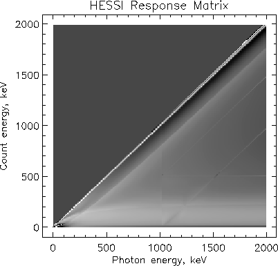
Figure 18 shows a full response matrix in greyscale. A vertical slice through this plot gives the spectral response to photons of a single energy (i.e. one of the traces in Figure 17).
The various energy-dependent contributors to instrumental response are listed in Figure 14. The response matrix software calculates the full response (Figure 18) by calculating each of these ``submatrices'' separately and then either multiplying them together (for the diagonal or photopeak parts) or adding them in (for the off-diagonal or scattering parts). This is done by the master response-matrix building routine, hessi_build_srm.pro (q.v.). When some of the submatrices are time-consuming to build and can be reused (for instance attenuator transmission will never change throughout the mission), they can be separately stored to disk and hessi_build_srm can be instructed to read them from disk instead of regenerating them. The submatrices which affect photopeak efficiency are:
Grid transmission: this cannot be simulated, because
the transmission of a grid pair is a strong function of the exact
shape, regularity and alignment of the slats. The grid transmission
submatrix is derived directly from laboratory measurements at the
x-ray and optical grid calibration facilities at GSFC. It uses
transmission averaged over a half rotation (which is equivalent to
a full rotation by symmetry).
| Attenuator transmission: The attenuator state
(none, one, or both in place) is of course a necessary input to
the response matrix software. It is available in housekeeping
data. You should not attempt to take spectra in a long time
interval containing more than one attenuator state unless your
only interest is in high energies (well above 100 keV) where the
attenuator has little effect.
| Blanket transmission: There are layers of
thermal blanketing above and below the imager, above the spectrometer,
and inside the spectrometer. They are virtually transparent above
10 keV but are important for the lowest energies. The beryllium
windows in the cryostat are included here, but are even more transparent
than the blanketing due to their very low atomic number (thus low
photoelectric cross-section).
| Detector efficiency: Photons which enter the detector
with their full energy can, at high energies, go right through,
or else leave less than their full energy (for a photopeak
efficiency correction these are equivalent). Most frequently
the photon will Compton-scatter out, but annihilation photons,
germanium K-shell fluorescence photons, or even Compton- or
photo-electrons can also escape.
| Electronic threshold cutoffs: The slow LLD must trigger
in the front segment in order for an event to be produced, and in the
rear segment both the slow and fast LLDs must trigger (see above).
These requirements produce a low-energy cutoff in the spectrum just as
the blankets and attenuator do. Because of the finite resolution of
the electronics, these cutoffs are not sharp and the loss of events
they produce must be compensated for just like any other absorption in order
to get the proper spectral shape below 10 keV (fronts) or 30 keV
(rears).
| |
The effects that produce off-diagonal (non-photopeak counts) are:
Scattering in the detector: This is actually part of
the same submatrix as Detector efficiency above, and consists
of those photons which enter the detector with their full energy but
don't leave it all.
| Scattering in the spacecraft: For this component we
simulate photons on all paths except those which could
possibly interact with the detectors first. Thus there can be
no photopeak events, since any photon which hits the detectors
must have Compton scattered first. Many of these photons are
stopped by the graded-Z shielding on top of the cryostat, but
they are still significant, particularly in the rear segments
at relatively low energies (below 200 keV). There is relatively
little contribution above a few hundred keV due to the nature of the Compton
formula: since most of the photons have undergone a large-angle
scatter before hitting the detector, they have usually lost the
majority of their energy.
| Scattering in the grids and attenuator: Photons which
scatter in the passive material above the detectors can contribute to energies below but near the photopeak, since they
can hit the detector after a small-angle scatter. In addition,
this submatrix will include the fluorescence photons from the
grids mentioned above. We are only simulating scattering of
photons in the lower grid, since a photon which scatters in
the upper grid has a relatively low chance of hitting a detector
due to the large distance.
| Scattering in the Earth's atmosphere: Since the rear
detectors have only a little aluminum between them and space on the
sides (and only somewhat thicker aluminum behind them), many flare
photons Compton-scattering off the atmosphere will be counted (these
are sometimes called albedo photons). In fact, we expect these
photons to dominate the rear segment count rate in medium to bright
flares (for weak flares, it is dominated by background). They will be
even more likely than spacecraft-scatter photons to have gone through
large-angle scatters and multiple scatters, so they will be soft
(mostly < 100 keV). We simulate this effect by a two-part
Monte Carlo. We first bounce simulated flare photons off a simulated
spherical atmosphere, recording what spectrum comes from it as a
function of position around the Earth and angle from the zenith.
We then convolve this matrix with another, the output of a simulation
of the spectrometer's total response to photons at various energies
and various (large) angles from the solar direction. In order to
use the resulting submatrix properly, you must provide the Sun-Earth-HESSI
angle (or a distribution of angles).
| |
The finite energy resolution (line shape) is also an effect that moves counts away from the energy of the input photon. For continuum work its effect is negligible, since it only moves energies a small amount. For work with narrow lines, it's often useful to know the best current guess at the instrumental line shape, so as to see whether a solar line is genuinely broadened. The line shape is a convolution of two submatrices: the intrinsic lineshape from the detector and the noise introduced by the electronics. The electronic noise is independent of line energy, usually symmetrical, and often Gaussian. It can be independently measured by turning on the pulser occasionally (see above). The intrinsic noise has a Gaussian component proportional to the square root of energy (due to counting statistics of the electron-hole pairs) and the trapping component, linearly proportional to energy (see Figure 13). Both the intrinsic and electronic lineshapes may change so fast that the database for the spectroscopy software cannot always keep up. To be sure you understand the instrumental lineshape, you can look at the shape of background lines during non-flare times. Most background lines are narrow, although the 511 keV line from the Earth's atmosphere has its own width of 2 or 3 keV.
Please keep an eye on the HESSI web pages for future revisions of this
document. If you have any questions on these topics, please contact
me at the email address above. For questions on the mechanics of the
spectroscopy software, contact Richard Schwartz
(Richard.Schwartz@gsfc.nasa.gov).
![]()
| About this document ... |
![]()

