The starting point of forward-fitting is the estimation of source centroid
positions from an initial back-projection map. For the standard example,
we obtain a back-projection map by:
o = hsi_image()
o -> set,image_algorithm='back_projection'
im = o -> getdata()
o -> plot
p = o -> get()
print,p.det_index_mask
.... e.g. [0,0,0,1,1,1,1,1,0,...]
print,p.image_dim
.... e.g. [64,64]
print,p.pixel_size
.... e.g. [4",4"]

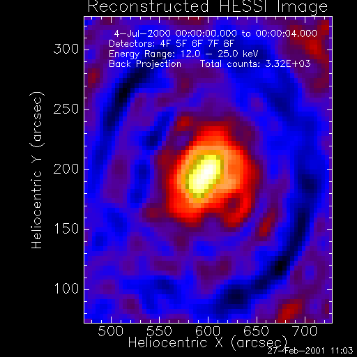
The back-projection map shows a compact source that does not resolve the two gaussian
source components used in the simulation of the data. Therefore, if we start forward-
fitting from such an unresolved back-projection, no good initial guess of the two
true source centroid positions can be made. However, if the resolution is increased,
the two souces can be resolved in the back-projection map. It is therefore advisable
to optimize first the pixel size. If we keep the same computational effort (which scales
with the image size nx*ny), the field-of-view will be proportionally smaller to the
smaller pixel size. One should be careful to chose the field-of-view sufficiently large
to encompass the areas of significant emission. Here, the source is so compact, that
we can decrease the field of view and pixel size by a factor of 4. Note also that the
default setting of the detectors excludes the finest 3 detectors and the coarsest
detector. In order to take advandate of the finer spatial scales we should include
finer detectors, e.g. # 3.
o = hsi_image()
o -> set,image_algorithm='back_projection'
o -> set,image_dim=[64,64]
o -> set,pixel_size=[1,1]
o -> set,det_index_mask=byte([0,0,1,1,1,1,1,1,0])
im = o -> getdata()
o -> plot

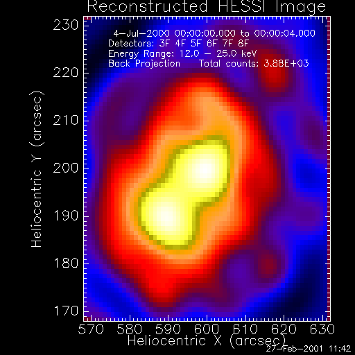
The two source components appear now to be resolved in the backprojection map.
This is a good starting point for forward-fitting. So we use the same image size
and pixel size to start forward-fitting, and specify 2 gaussian components
(because the default is 1):
o -> set,image_algorithm='forwardfit'
o -> set,n_gaussians=2
im = o -> getdata()
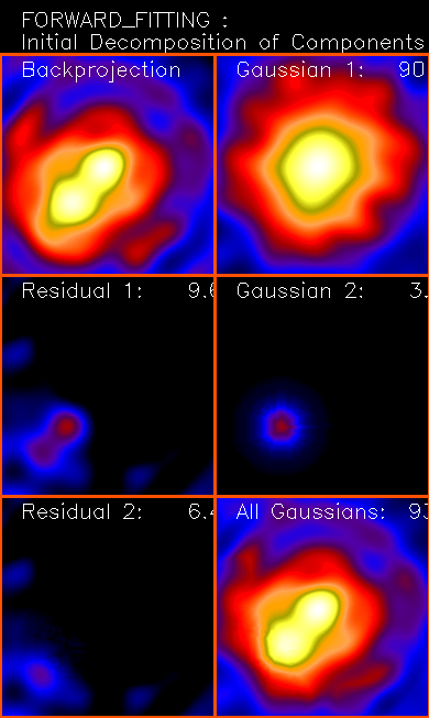
The decomposition of the backprojection map in the forward-fitting algorithm
is displayed on the screen (if the keyword TESTPLOT is enabled, which is the
default):

The position of the first gaussian component is measured from the global maximum in the backprojection map (top left) and a backprojection of the first gaussian is calculated (top right), and then subtracted from the original backprojection map. From the residual map (middle left), the global maximum is determined as initial guess for the second gaussian (middle right). The second gaussian is subtacted again and the next residual map is shown (bottom left). The sum of the two separated backprojection map is also shown (bottom right), which should look similar to the original backprojection map (top left).
If one does not succeed to resolve closely-spaced sources in the initial backprojection map, the set of detectors can be reduced to accomodate for the optimum spacing, e.g. by selecting those detectors that match the source separation and their instrinsic width.