Without any a priori knowledge we would first attempt to fit the data with a
single gaussian component:
o = hsi_image()
o -> set,image_algorithm='forwardfit'
o -> set,n_gaussians=1
o -> set,image_dim=[64,64]
o -> set,pixel_size=[2,2]
o -> set,det_index_mask=byte([0,1,1,1,1,1,1,1,1])
im = o -> getdata()
o -> plot
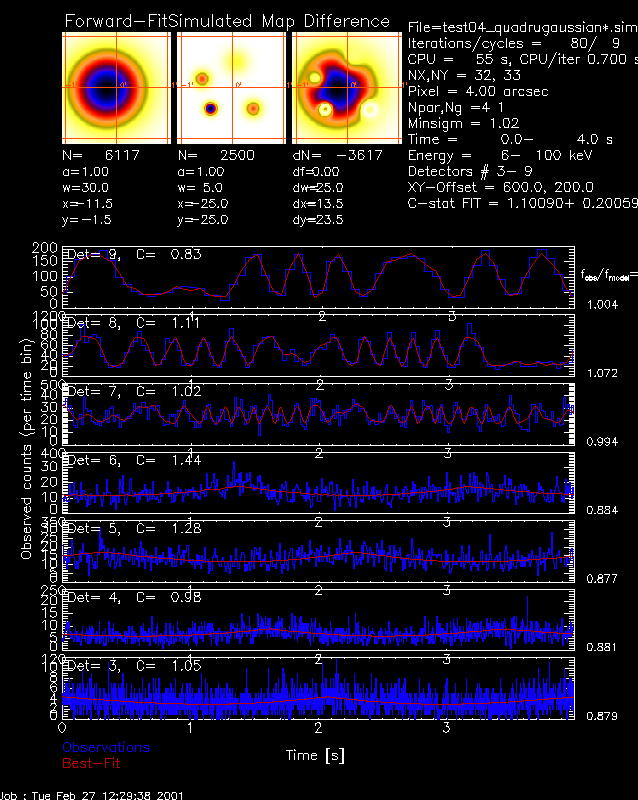
The average value of the C-statistic has a value of C=1.10, which is not too
bad, because the centroid of the 4 sources produce a similar modulation as the
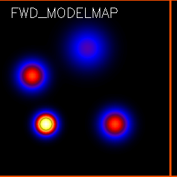
sum of the 4 sources. However, the total flux (6117/s cts) deviates strongly
from the modelmap (2500 cts/s), which does not affect the C-value (in the
current renormalization). Because a value of C>1.05 is considered not as
best possible fit, we increase the number of sources to two:
o -> set,n_gaussians=2
o -> set,det_index_mask=byte([0,1,1,1,1,1,1,1,1])
im = o -> getdata()
o -> plot
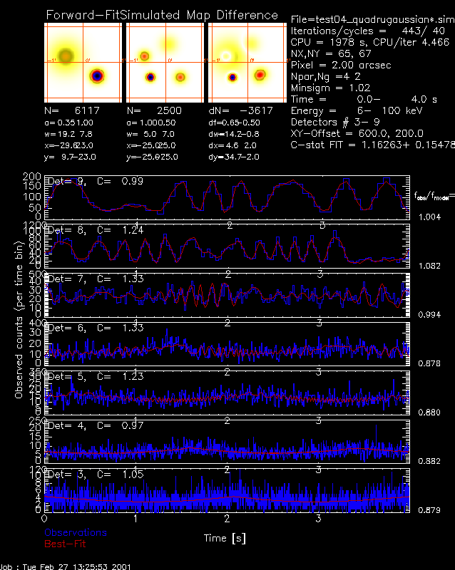
The fit with two gaussians yields a C-statistic of C=1.16, and a disagreement
in the count rate of N=6117 cts/s instead of N=2500 cts/s. Because a value of
C<1.05 is expected for a best possible fit, we increase the number of sources
to three:
o -> set,n_gaussians=3
o -> set,det_index_mask=byte([0,1,1,1,1,1,1,1,1])
im = o -> getdata()
o -> plot
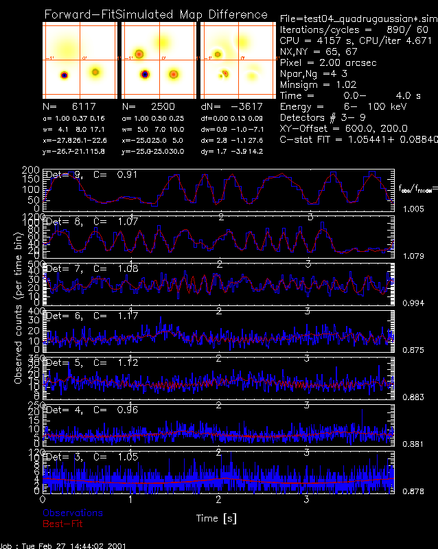
The fit with three gaussians yields a C-statistic of C=1.05.
We increase now the number of sources to four. Sometimes, a sidelobe of a source component
occurring in the backprojection map may confuse the location of the true sources, even if
they are well-separated. In such cases, the setting of a requirement on the minimum separation
distance between sources may help [e.g. image=o->getdata(image_algorithm='forwardfit',minsep=30)].
o -> set,n_gaussians=4
o -> set,det_index_mask=byte([0,1,1,1,1,1,1,1,1])
im = o -> getdata()
o -> plot
