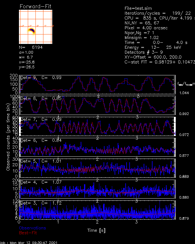
Source structures with geometries of spherical gaussians and elliptical
gaussians can be simulted with the so-called (predefined) "gaussian source structure":
model = {gaussian_source_str}
model.amplitude = 1.0 ... (normalized amplitude)
model.xysigma = [4.,4.] ... (gaussian widths in x- and y-direction in arcseconds)
model.xypos = [3.3,6.6] ... (offset in x- and y-direction from map center XYOFFSET)
model.tilt_angle_deg = 0.0 ... (tilt angle of ellipse)
The structure can also be defined by the following syntax:
model = {gaussian_source_str, amplitude:1.0, xysigma:[4.,4.], xypos:[3.3,6.6], tilt_angle_deg: 0.0 }
model = {gaussian_source_str, 1.0, [4.,4.], [3.3,6.6], 0.0 }
or replicated for a double source:
model2 = replicate( {gaussian_source_str} , 2)
The next steps to setup a simulations involve definitions of
the photon rate [photons/s/collimator], the offset of the simulated
and reconstructed map center, the simulated and reconstructed energy band.
Then we run an image reconstruction with forward-fitting, yielding the
image im, extract the parameter structure p, and display the image with
the plotmanager.
o=hsi_image()
o->set,sim_model=model,sim_pho=5.0e4
o->set,sim_xyoffset=[600.,200.],xyoffset=[600.,200.]
o->set,sim_energy_band=[12.,25.],energy_band=[12.,25.]
o->set,det_index_mask=bytarr(9)+1B
o->set,image_algorithm='forwardfit'
im=o->getdata()
p=o->get()
o->plotman

You might be interested to verify how good the forward-fitting retrieved the
model parameters:
p = o -> get()
print,p.ff_coeff_ff
.... coefficients of forward-fit, e.g. [1.00, 6.69", -25.79", -26.49",2.01,59.20,0.26]
The definitions of the 7 coefficients are:
print,p.ff_coeff_ff(0)
.... amplitude a= 1.00
print,p.ff_coeff_ff(1)
.... gaussian width w_x=6.69" "
print,p.ff_coeff_ff(2)
.... x-position x=-25.79""
print,p.ff_coeff_ff(3)
.... y-position y=-26.49""
print,p.ff_coeff_ff(4)
.... eccentricity e=w_x/w_y-1=2.01 -> gaussian width w_y=w_x/(1+e) "
print,p.ff_coeff_ff(5)
.... tilt angle in degree t=59.20
print,p.ff_coeff_ff(6)
.... curvature parameter c=w_x/r=0.26 -> curvature radius r=w_x/c=
The comparison with the model parameter yields:
print,model.amplitude, p.ff_coeff_ff(0)
.... 1.0, 1.0
print,model.xysigma(0),p.ff_coeff_ff(1)
.... 5.0", 6.7"
print,model.xysigma(1),p.ff_coeff_ff(1)/(1+p.ff_coeff_ff(4))
.... 1.0", 2.2"
print,model.xypos(0),p.ff_coeff_ff(2)
.... -25.0", -25.8"
print,model.xypos(1),p.ff_coeff_ff(3)
.... -25.0", -26.5"
print,model.tilt_angle_deg,p.ff_coeff_ff(5)
.... 60.0 deg, 59.2 deg
print,model.curvature,p.ff_coeff_ff(6)
.... 0.20, 0.27