Brian Dennis
Last modified 12 January 2004 - added reference to hessi_spex
This is a beginner's guide to RHESSI spectroscopy. It assumes that you have already set up your computer to run IDL (Version 5.3.1 or later, preferably 5.4 or 5.5) with the Solar Software (SSW) tree and with access to the RHESSI flight data (see Software Installation Instructions and Accessing HESSI Data). It will take you through demonstrations of the RHESSI Graphical User Interface (GUI) to the RHESSI software and the SPectral EXecutive (SPEX) package. A detailed SPEX Help document called Analyzing Flare X-ray Spectra Using SPEX is available in SSW. It includes comments on an interactive session at the command line, and a description of the available user commands and parameters. A follow-on to this First Steps document called RHESSI Spectroscopy - Second Steps has been written by Linhui Sui and Astrid Veronig and provides instructions for the more advanced capabilities of SPEX. Another guide to RHESSI spectroscopy using the IDL command-line interface has been written by Chris Johns-Krull.
The objective of this document is to demonstrate how to obtain spectra of the total solar photon flux incident on the RHESSI instrument for different time intervals during a flare. Imaging spectroscopy is not covered in this demonstration; further analysis is required to obtain spectra for different areas within an image.
The GUI is a user-friendly way to obtain light curves, images, and count-rate spectra. Currently, it can also use the diagonal elements of the instrument response function to produce so-called "semi-calibrated" photon flux spectra but without subtracting background.
SPEX takes as its input the count-rate spectra produced by the GUI (or by this IDL command-line input). (See Chris Johns_Krull's Overview of the Command Line Interface for HESSI Data Analysis Software.) SPEX defines the time intervals for analysis, determines and subtracts the background, decides on the functional form to assume for the photon spectrum, and uses the instrument response function to produce photon flux spectra. The user must provide guidance to SPEX at each step in the process as will be evident in this demonstration.
First, let's produce a semi-calibrated spectrum using only the Graphical User Interface (GUI) , and using simulated data. Enter IDL so that it uses SSW and has access to the RHESSI flight data. You should see the following standard prompt in the IDL window:
IDL>
To enter the GUI, simply type the following after this prompt:
hessi
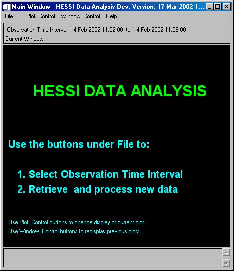
You should get a window that looks like this:
We begin by choosing the observing time interval containing the flare of interest. For this demonstration, we have chosen a flare that occurred on February 20 at 11:00 UT. The selected interval includes time before and after the flare to allow good background spectra during the flare to be obtained.
On the command bar at the top of the GUI window, pull down "File" and choose
Select Observation Time Interval
A new window will open similar to the one shown below. It allows you to select data by date and time, by looking at RHESSI's flare list, by picking a flare by number, or by looking at the Observing Summary data and picking a time interval from the overall light curve.

We will do it by specifying the start and end times. You can type them directly into the "Start..." and "End..." windows or you can click the "Start" button and enter the following date and time in the window that opens up:
Year 2002, Month February, Day 20, Hour 11, Minute 0, Second 0
Click the "READY" button and the following should appear in the "Start" location of the Observation Time Selection Window:
20-Feb-2002 11:00:00.000
You can enter the end time in the same way by pressing the "End" button or you can click on the "Duration (s)" box and edit its contents by typing "3600" over whatever is already there. You must then press the "Enter" key and the following end date and time should appear in the box next to the "End" button:
20-Feb-2002 12:00:00.000
The Observation Time Interval Selection window should now look like the following:
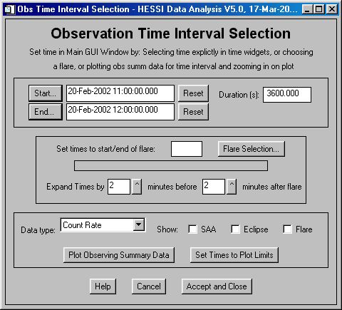
Once the correct Start, Duration, and End dates and times appear in the respective boxes, click the Accept and Close box to exit back to the opening GUI window.
Now let's look at spectra. Back on the main GUI window, use the pull-down menu on the top to select:
File ------- Retrieve/Process data ---------- Spectrum
and a new window labeled SPECTRA should open up looking something like the following:
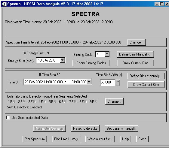
Note that both the Observation Time Interval and the Spectrum Time Interval shown in this window are the same as previously selected. We must select the time intervals within this overall time for spectral analysis. The flare of interest is finished by about 11:20 UT so we will change the spectrum time interval to end at that time. Click on the "Change..." button and set the interval duration to 1200 s and return.
We now want to divide the flare up into useful time intervals. We must also be sure to select some intervals, both before and after the flare if possible, that can be used for background determination. The default is to divide the Spectrum Time Interval into equal one minute intervals. The default time bins can be changed by pressing the "Define Bins Manually" button in the third box down from the top of the window where the current Time Bins are listed in the pull-down box. For now we will accept the default of 20 intervals each 60 s long.
Next we must decide what energy bins to use for our spectra. This is done using the second box from the top that initially lists the default energy bins for Binning Code 7.. Generally you want to pick energy bins fine enough to distinguish between the different emission models you want to study, but not so fine that the statistical noise is overwhelming. Binning Code 7 gives bins that are a bit coarse for detailed continuum spectral work (such as separating out thermal, superhot thermal, and power-law components, for instance). There are several other good default choices, or you can construct your own binning by pressing the "Define Bins Manually..." button. You can see what default energy bins are available by clicking on the "Show Binning Codes" button. We will use one of the other default sets by selecting Binning Code = 1. To do this, click on the pull-down menu next to the words "Binning Code" and select "1." Binning Code 1 gives us 1-keV bins from 3 keV up to 100 keV.
Keep in mind that the total number of bytes of memory Nb that you will need to store all of these spectra depends on the number of time bins Nt and the number of energy bins Ne that you specify according to the following relation:
Nb = Nt x Ne x 432 bytes
In our case, Nt = 20 and Ne = 97, so we will only use up 838 kbytes. For more detailed analysis, you will want to choose finer time bins as short as half a rotation or about 2-s long but you must be careful not to choose too many time intervals and energy bins so that Nb exceeds the available memory space.
The next panel lets us select detector segments: front and rear for any or all of the 9 detectors. The document Behind, Beneath and Before HESSI Spectroscopy or "BBB" discusses the detector segments in detail. Basically, the front (F) segments detect most of the hard x-rays up to 100 keV and the rear (R) segments detect most of the gamma-rays above 100 keV. The flare we are analyzing is only detectable up to 100 keV so we choose just the front segments. This is the default setting.
We should also do something that you'll probably want to do most of the time in real life: remove from consideration the front segment of the detectors under Grids 2 and 7. (We refer to these detectors as "G2" and "G7" for short). Detector G2 after the first couple of weeks in orbit could only be used in the unsegmented mode and has a resolution of about 10 keV and a threshold energy of about 25 keV. Detector G7 has an energy resolution in its front segment of about 3 keV instead of the ~1 keV FWHM at hard x-ray energies that the other detectors have. To deselect these two detectors, click on the "Change" button in the fourth box down in the Spectra window that shows the selected detectors and segments. A new window appears that allows you to select or deselect any segment. Click on the checked boxes next to 2F and 7F to deselect them. Note that all the other front segments are selected and all the rear segments are deselected. Click on the "Accept" button to return to the Spectra window.
You should also be aware that Detector 8 also has problems when the transmitter is on and is using the aft antenna. There is some noise pickup that results in a higher background at these times in this detector channel. You can check for this by plotting the light curve for this detector alone and comparing it with the light curves for the other detectors. We don't have to worry about it for this flare.
At this stage the SPECTRA window should look as follows:
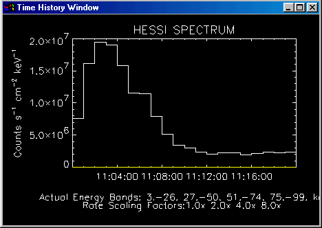
We can see the time history of the flare we are analyzing by pressing the "Plot Time History" button at the bottom of the SPECTRA window. Note that since this is the first time we are actually extracting the information about individual counts from the flight data files, it takes a little while for this step to execute - about 2 minutes on my 800-MHz laptop. The actual time taken depends on the number of counts recorded in the interval of interest. So depending on the speed of your computer you must be patient. It's a good idea to have the main IDL window visible before you click on this button so that you can see any error messages in case the program crashes. You can generally tell if everything is going OK by noting occasional disk activity while you are waiting. The time history for this flare will appear in the main GUI window and look like the following:
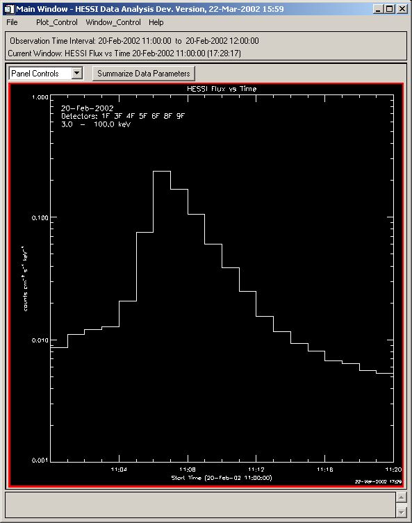
This is the counting rate time history summed over all the energy bins we selected. You can view the light curve for any individual energy bin or any group of bins, either separately or summed by clicking on the "Plot_Control" pull-down menu and select "XY-Plot Display Options." In the resulting window, you can also change the appearance of the plot such as switch to a linear scale or change the maximum and minimum values of the Y-axis.
Once you are satisfied with the appearance of the time history plot, close the XY-Plot Options window.
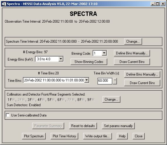
Now let's look at the spectrum we're getting by pressing the button on the bottom of the SPECTRA window labeled "Plot Spectrum." The result will appear in the main GUI window and should look like this.
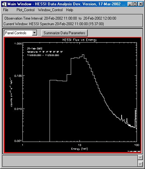
This is the count spectrum, meaning it's the spectrum of the detector counting rates vs. the energy that the detectors recorded for each count. It is summed over all of the time intervals that we selected. Again, you can plot any one or a selected group of intervals by clicking on the "Plot_Control" pull-down menu and select "XY-Plot Display Options" as before.
First, notice that the spectrum is rising from 3 to about 12 keV. This is not a characteristic of the Sun; it's due to absorption in passive material in front of the detectors (thermal blankets, beryllium detector windows, and most importantly the aluminum attenuators, the thinner of which was in place for this flare). From 12 keV to 100 keV the spectrum falls roughly as the true solar spectrum does. The background spectrum contributes a greater fraction of the total at the higher energies. Also, the sharp peaks that can be seen in the spectrum at energies above 50 keV are lines from the germanium detectors and are not of solar origin.
The rest of this document will be devoted to converting this count spectrum to a photon spectrum, i.e. what's incident on the spacecraft from the Sun. The simplest thing to do is to divide this spectrum by the efficiency of the system as a function of energy. This will remove the effects of absorption from the materials in front. To do this, simply click on the check box next to "Use Semi-calibrated Data" and then click on the Plot Spectrum button again. You should now see something like this:
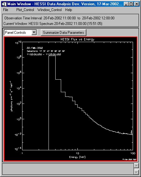
The instrumental absorption which caused the spectrum to roll over below 12 keV is gone. Unfortunately, the background is still not subtracted and the flattening at higher energies above ~30 keV is not real. Later versions of this program will allow the background to be computed and removed before the photon spectrum is computed. The slight bump at 6 - 7 keV is probably the real iron-line feature from the flare.
"Semicalibrated" photon spectra of the type shown above can be used with caution for science when all of the following conditions hold:
To determine the incident photon spectrum more accurately, we must use the full Spectral Response Matrix (SRM). (Note that this is called the Detector Response Matrix or DRM in SPEX). Each line of the SRM gives the total response of the instrument to photons of a particular energy. The diagonal terms of this matrix represent the total system efficiency for recognizing a photon energy directly. Off-axis elements represent the probability that photons are redistributed to another (generally lower) energy. For hard x-rays, more photons are recorded with their true energy than with a lower energy, but above 100 keV this is reversed. This is why the "semicalibrated" procedure, which simply takes the diagonal elements of the response and divides the count spectrum by them to get a photon spectrum, is inaccurate above 50-100 keV or so, even without considering the issue of background. Note also, that using only the diagonal elements gives inaccurate results below 10 keV if either shutter is in the FOV because of the germanium K-shell escape events.
To analyze count flux data in SPEX, a count rate spectrum and a response matrix must be read into the active session. The response matrix is stored in the array drm within the SPEX common blocks. When using the HESSI spectrum object or GUI to create the count rate spectrum file and response matrix file ( filewrite on the CLI and write output from the GUI), the name of the response matrix file is written in the RESPFILE parameter in the header of the spectrum FITS file. A different drm is needed to analyze the count rate obtained with each attenuator state.
The way we are using the HESSI spectrum object right now, you only need one srmfile for each attenuator state for each detector combination for every binning, specify that with dfile, and then use read_drm to create the drm array used with SPEX. There is no distinction by flare at this time even though we autoname the srmfile with the flare date and time, 11/15/02. In the future there will be some information about the average position of the source from the imaging axis. You can even write all of the spectrum data for a flare into one file and then change the drm as needed. I recommend that you adopt a standard binning code and a standard set of detectors and create srm files for all three of the used attenuator states. Then you should name the srm files to something like hsi_srm_generic_bincodeX_detZZZZ_attN.fits. X would be the binning code (one of those from the GUI or your own system), ZZZZ would indicate your choice of segments, and N would indicate the attenuator state. You can produce these srmfiles from the spectrum object (sp_obj->filewrite,/fits,/build,... ) or from the SPECTRUM GUI by choosing a start time when the instrument is in the needed attenuator state.
Now let's do more accurate spectral analysis using SPEX. First we'll make some files for SPEX to use. Let's go back to the SPECTRA window and click on the box next to "Use Semi-calibrated Data" so that the check disappears.
Now we can create and save two FITS file for SPEX to use. The first will contain a time series of spectra, one for each of the 20 time bins, with 97 energy bins in each spectrum. The second FITS file will contain the SRM of the instrument for the specific time of this flare. To do this, click on the button labeled "Write output file..." at the bottom of the SPECTRA window. The following window will appear:
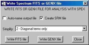
The "Create SRM file" is checked by default but we need to decide if we want to use just the diagonal terms, an approximation of the off-diagonal elements, or " the "full calculation of off diagonal, diagonal elements" from the pull-down list of choices next to the word "Simplify." For now, to speed up the demonstration and since the flare we are analyzing is detectable only up to about 100 keV, we will leave it set at the default choice of "2- Diagonal terms only." Also, since the thin shutter was in place at this time, we will limit the analysis to >10 keV.
Now go ahead and click the "Write FITS file" button.
It will offer you the following file names (based on the start date and time) for the spectrum and srm files, respectively:
hsi_spectrum_20020220_110000.fits
hsi_srm_20020220_110000.fits
You may accept these and put them in your default IDL Working Directory or you can enter different paths and/or names to save them in a different directory. Be sure to use the same file names and locations when you enter SPEX. When the box that says "Working..." disappears, you may click on the "Close" button in the "Write Spectrum FITS or GENX file" window.
Now let's start SPEX to produce a more accurate photon spectrum and obtain best-fit function parameters for the time intervals we have selected.
SPEX is completely independent from the GUI but the experts tell me that, just to be on the safe side, it's a good idea to close the GUI before you start SPEX so that there is no chance of any interference.
SPEX has its own independent command structure within the IDL/Solarsoft environment.
To start SPEX, type the following in the IDL command line after the IDL> prompt:
hessi_spex or
spex_proc
The "hessi_spex" procedure was created in November 2003 to initialize SPEX with the defaults suitable for RHESSI analysis. The "spex_proc" procedure starts SPEX with initialization suitable for BATSE analysis. The parameters that are initialized differently are data_tipe, flare, and _1file (see the parameter list and explanation below).
SPEX will put up two blank windows, one called the "Time History Window" the other the "Spectrum Window." It displays the following prompt in the IDL window:
SPEX>
At any time in SPEX, type "list" in the IDL command line
to display a listing of all the commands that are available to SPEX and all the
parameters that can be changed.
Type "?,command" without the double quotes at
any time to get an explanation of "command."
Change options by entering item,
comma, new value. After setting options, enter one of the available commands.
Parameters and commands only need the shortest unambiguous abbreviation to be
typed.
They may be strung together by inserting !! between entries. To delete
a string field, place a '' in the field.
There are two ways to obtain a printed version of any plot that SPEX generates. One way is to click in the window containing the plot and then press the Alt and Print Screen keys simultaneously. This will save a copy of the window in your Clipboard so that you can paste it into any program that can handle images (Word, PowerPoint, Irfanview, etc.) and generate a graphics file of the desired type. You can also produce a postscript file of the most recently generated plot with the create_ps command. To make it reproduce the plot in color, you need to enter the following two IDL commands first from within SPEX:
idl,sps,/color
A postscript file is created in your IDL working directory with a name like "count_spectrum_100330_212509.ps" that can be displayed and printed using Ghostscript. To get such a postscript version into the standard image handling programs, you need Adobe's Distiller program to convert it into a pdf file and then Acrobat to extract the images to the Clipboard again.
If you should enter a command that causes SPEX to crash, you can almost always recover by typing "retall" at the IDL prompt and then restating SPEX using "spex_proc" or "hessi_spex" as above. Generally, SPEX remembers where it was before the crash and you can continue on with the analysis.
You can always save your work to date by typing the command "save_event." Two files called summary.dat and spex_dflts.dat are written to your IDL working directory. They can be read back in by typing the command "restore_event."
First, type "list" in the IDL command window. You should get the following list of all the the commands that SPEX recognizes and all the parameters that can be changed at this point in the analysis. We show the parameter values for the hessi_spex procedure:
Spectral Analysis Executive (SPEX)
START_TIME_DATA
END_TIME_DATA
QUIET 1
CHECK_DEFAULTS 1
DFLTS_FILE spex_dflts.dat
DATA_TIPE hessi allseg_1FILE hsi_spectrum*.fits
_2FILEDIRECTORY
FLARE 665
DET_ID 1
COSINE 0.000000
SOURCE_RADEC 0.000000 0.000000
PSSTYLE PORTRAITCommands: /drm /fitting /interval /summary /time_history ? batse_menu comments erase execute exit
find_files hard idl initialize kleanplot list merge_batse online? preview pspreview reset_event
restore_dflts save_dflts script steps_help stop tek zoomAdditional commands: / accum background_interval bspectrum build_drm cal_restore cal_save ch_bands
clear_ut count_spectrum create_ps display_intervals enrange fitting force_apar graph multidrm
nospec_bands photon_spectrum read_drm recalibrate restore_event save_event select_interval
spec_bands t_hist_mode time_historyChange parameters or enter a command
Note that the commands that start with "/" put you into different sections of SPEX with additional command options. Once in the new section, you can always type "list" again to see the new set of commands that apply there. You get back to the starting section with the "/" command.
First, we'll tell SPEX that we're using RHESSI front-segment data:
data,hessi,front(other options are rear or allseg). "hessi_spex" initializes the data_tipe parameter to hessi,allseg so this step may not be necessary. If you had selected rear-segment data or both front and rear when creating the input file, you would type data,hessi,rear or data,hessi,allseg respectively.
Now we'll tell it to read in the spectral file ("_1file") and response matrix file ("dfile") that we just created. You can cut the file names from your IDL working directory, where the GUI puts them by default, and paste them into the IDL command line. If the files are not in the IDL working directory, then you must give the full path name.
_1file, hsi_spectrum_20020220_110000.fits
dfile, hsi_srm_20020220_110000.fits
Note that filenames do not require quotes. If the value of _1file contains a wildcard ("hessi_spex" initializes it to hsi_spectrum*.fits) then typing the preview command will display an interactive widget that lets you select a file from a list.
You can preview the data to make sure that SPEX knows where to get the data and response matrix from as follows:
preview
This should give the following response if everything is OK:
File C:\IDL_WORKING_DIRECTORY\hsi_spectrum_20020220_110000.fits found.
Data will be read from C:\IDL_WORKING_DIRECTORY\hsi_spectrum_20020220_110000.fits
Data file name returned: C:\IDL_WORKING_DIRECTORY\hsi_spectrum_20020220_110000.fits
Change parameters or enter a command
SPEX>
To plot a time history of the data that have been read in, enter
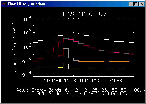
graphYou should see a similar count-rate time history in the time history window that we saw in the GUI.
The default here is a linear scale. I prefer to display the count rate on a log scale so that you can more clearly see when the flare starts and ends, and when would be good intervals to choose for the background, particularly at the higher energies. This can be changed to a log scale by typing
th_ytype,1
th_yrange,1.e-4,1.e3
The last command adjusts the Y axis to match the range of fluxes plotted by changing the array th_yrange. The first number is the lower limit on the flux being plotted and the second number is the upper limit. Note that to see these parameters and verify that the changes have been accepted, you need to go to the time history section of SPEX by typing
/time
list
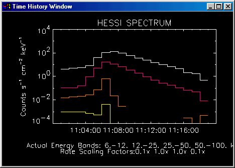
Four default energy bands will be plotted. These can be changed to the more standard bands by typing the following:
energy_bands, 6,12,12,25,25,50,50,100
Change the multiplication factors that will be used for each band with the following command:
scale_bands,0.1,1,1,0.1
Then, after typing "graph" you should see following time history:
Now let's create the background spectrum by telling SPEX to accumulate it during intervals before and after the flare when there is nothing going on. This won't always be possible, but when such intervals exist within 10 minutes or so of the flare it's usually the best way to get an accurate background measurement. SPEX can fit a polynomial background model of order N for each energy bin given at least N background time intervals.
Initially, we will choose one background interval before the flare and one after it is over. We will then choose to linearly interpolate (order one) between the spectra in the two intervals in order to arrive at a background spectrum to subtract at each time interval during the flare. If you have more background intervals, then you can fit them with a higher order polynomial to try and get a better estimate of the background during the flare. Also, you can use different background intervals for four different energy ranges to better estimate the background, particularly at higher energies where the flare duration is shorter. This technique is described below but for now, to keep it simple, we will just choose one interval before the flare and one afterwards and use them globally for all energies.
First, set the order of the interpolation polynomial to one -
back_order,1
Then, to choose background intervals before and after the flare, first type
background
The following window will appear:
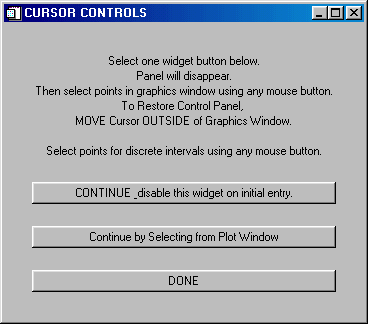
Click on the "Continue by Selecting from Plot Window" button.
Then move the mouse over the window with the active display ("Time History Window"). Push the left mouse button to define each side of the time intervals to be used for background determinations. Choose the first interval inside the first 1-minute interval of the time history and the second interval inside the last 1-minute interval. Note that the left edge will automatically revert to the data interval to the left of where you select; the right edge will revert to the next edge of a data interval to the right of where you select. Also, be careful that you don't click too fast. Wait after each click to see the vertical line appear on the plot and see the message appear in the IDL output log window. After clicking four times, you should see the following figure:
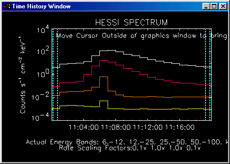
Once you have selected the two intervals for background determination, move the cursor out of the Time History Window and click "DONE" in the same CURSOR CONTROLS window shown above.
The time histories should immediately change as the background is subtracted for each time interval and energy range. The resulting figure is shown below.
Note that the resulting count rates are negative in some time intervals and energy ranges indicating that the background rate has been overestimated. We will not worry about that at this stage since we still have a positive signal at all energies in the time interval of prime interest at the peak of the flare.
Now we will select one data interval for which to analyze the spectra. More can be selected but for this demonstration, we are just interested in the spectrum of the interval with the highest flux. Each interval that you select should of course be exclusive of your background periods. Type on the command line:
select_interval
and the following window should appear:
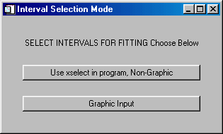
Click on the "Graphic Input" button.
Then the INTERVAL SELECTION window will appear as follows:
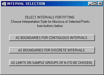
Click on the AS BOUNDARIES FOR DISCRETE INTERVALS button.
The selection of data analysis intervals is then the same as for selecting the background intervals. The same CURSOR CONTROLS window that used during background selection appears. Click on the "Continue by Selecting from Plot Window" button as was done for the background selection. Because we selected "discrete intervals", the first mouse click defines the start of an interval and the second defines the end. Again, remember to choose the interval "inside" the actual 1-minute data intervals to avoid selecting an interval wider than intended. I will do just 2 clicks to make a single interval and the figure will look like this, where you can see the time interval I have selected -
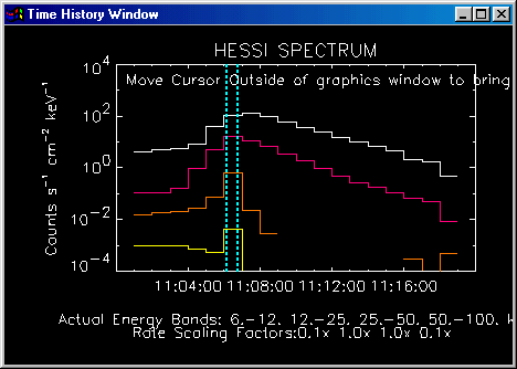
Next, move the mouse back out of the window and click on the "DONE" button in the CURSOR CONTROLS window.
Regraph by typing "graph" and then type "display" to show the selected time interval in theTime History Window -
Now SPEX has a background model, an instrument response, and a single time interval in which to accumulate spectra.
We must now go into the spectral fitting section of SPEX. Do this with the following command:
/fit
You don't actually have to type this command to execute the following commands and do the spectral fits but it has the advantage of allowing you to type "list" to see what values the various parameters have and what commands are available in this new section of SPEX.
The first thing to do is define the type of function you want to use for the fit. The default is a single thermal plus a broken power-law function, f_vth_bpow. This can be considered as the workhorse model because you can control the 6 free parameters in such a way that you can make it work as a single thermal, a single or a double power-law, or any combination of these functions. For this demonstration we will use it as a thermal plus a single power law by fixing the parameters of the higher energy power law so that it does not contribute significantly to the total flux in the energy range of interest below 100 keV.
The full list of available functions can be seen by looking at the procedure names in the Solarsoft distribution under packages/xray. You can read the documentation for each function by typing xdoc,' followed by the name of the function, e.g.
xdoc,'f_vth_bpow
You can get more information than you probably need at this point on the available functions by typing
xdoc,'model_components.pro
The workhorse function f_vth_bpow returns the differential photon spectrum seen at the Earth for a two component model comprised of an optically-thin thermal-bremsstrahlung function normalized to the Sun-Earth distance plus a non-thermal broken power-law function normalized to the incident flux on the detector.
a(0)= emission measure in units of 1049 cm-3
a(1)= KT plasma temperature in keV
For the "non-thermal" function it uses the broken power law function, F_BPOW.PRO:
a(2) - normalization of broken power-law at Epivot (usually 50 keV)
a(3) - negative power law index below break
a(4) - break energy
a(5) - negative power law index above break
a(6) - low energy cutoff for power-law, spectrum goes as E^(-1.5)
a(7) - spectral index below cutoff between -1.5 and -2.0
default parameters - a(6) and a(7) default to 10 keV and -1.5 can be overwritten by values in common function_com.
To see the spectra in count space before the fitting begins, enter
countand the neglected window comes to life.
The yellow curve is the flare count spectrum and the orange curve is the background. The white line represents the input photon power-law spectrum, and the green line is the thermal component. The blue line is the predicted count rate response of the detectors to that input photon spectrum. When the fit is complete, the blue curves should match the yellow, more or less. But for now, we have arbitrary values for the function parameters.
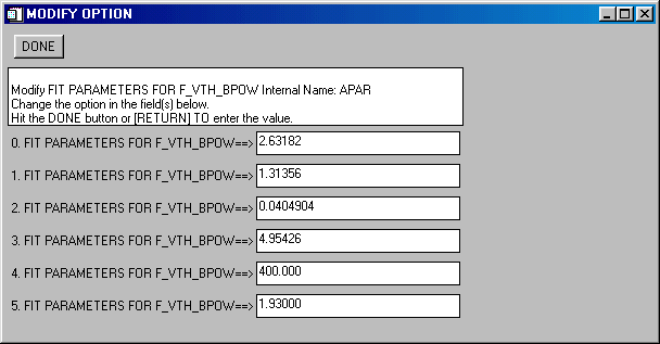
It is important to choose good starting parameters for the chosen function. For the interval we have used in this demonstration, good starting parameters are as follows:
apar,3,1.3,0.05,4,400,2
Note: Do not try to change these parameters with this command after doing the least-squares fit with the "fit" command. Instead, use the "photon" command as described below.
How would you choose these parameters yourself? One way is to start by choosing the first power-law parameters so that the function equals the measured photon spectrum at 50 keV and has about the right slope. Choose the other parameters such that the other components don't contribute significantly to the total function in the energy range of interest. Fix these other parameters with the "free" command introduced below and then do the fit. Once you have good power-law parameters, try estimating the thermal parameters you need to improve the fit at low energies. If you need a different power-law slope at higher energies, try guessing the required parameters for the second power-law function and freeing them prior to repeating the "fit" command. Finally, let all of the parameters of all the required components go free and obtain your final best fit.
The array "free" allows parameters to be fixed if the corresponding number is set to 0 or to vary if set to 1.We want to free the first four parameters and fix the last two as follows;
free,1,1,1,1,0,0
There are three ways now to select the energy bins to be included in any spectral fits in SPEX.
Use the two element parameter ERANGE. They are in the units of the energy bins (nominally keV).
Use the ENRANGE command to make a graphic selection of 1 or multiple ranges of energy bins.
Use the ENRANGE command with arguments, e.g. enrange, 10., 40., 60, 200. would select channels from 10-40 keV and 60-200 keV
For this demonstration we will keep it simple and use the ERANGE command to set the energy interval used in the fit to be 10 - 100 keV. This is done by entering the following:
erange,10.,100.
You can set this manually with the "enrange" command. This brings up a spectral window and allows you to click on the start and end of each energy range that you want to use. But to keep it simple, we will stick with 10 - 100 keV.
The f_vth_bpow function has a cutoff of the power laws such that below 10 keV, the power-law index is set to -1.5. This can be changed to 1 keV and -1.5 with the following command:
a_cutoff = [1.0,1.5]
where the first number is the cutoff energy and the second number is the power-law spectral index below that energy. Note the equals sign that allows SPEX to interpret this as an IDL command.
The SPEX command "fit" obtains best-fit spectra for all intervals between "ifirst" and "ilast." In our case since we have only selected one interval, both of these parameters are zero.
In preparation for showing the fitted spectrum and residuals, enlarge the Spectral Window to the full height of your screen. Before typing "fit" to obtain the best-fit spectra, it's a good idea to first type "list" and review carefully all of the settings and parameters. Otherwise, SPEX has a tendency to go into an unending loop if you have some parameter wrong, and the only recourse is to kill IDL and start SPEX all over again.
When you are ready, type "fit" to carry out the least-squares fit and determine the best-fit parameters that give the smallest value of chi-squared. After some calculations the following window appears:
You can see that we are getting a better fit between the blue curve (the predicted count spectrum) and the yellow curve (the measured count spectrum).
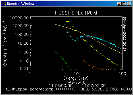
Then type "photon" to see the results of the fit. The following window will appear:
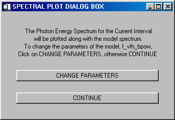
Click on the CHANGE PARAMETERS button in the resulting pop-up window to see the parameters used in the latest fit.
You can also change them for the plot and as starting parameters for a new fit. Clicking on the DONE button brings up a plot of the photon spectrum showing the data points and the different components of the fitting function using the newly changed parameters.
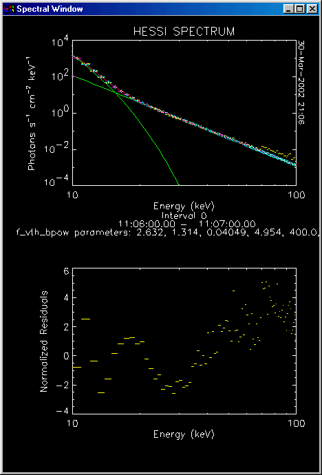
The best fit spectrum that I was able to obtain for our 1-minute time interval at the peak of the flare is shown below:
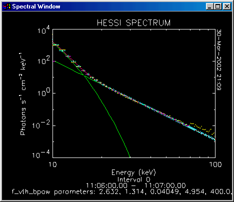
The plot shows the data points in yellow, the components
of the fitting function in green and the summed fitting function in red. The
best fit parameters are shown at the bottom. The thermal component has an
emission measure of 2.6 x 1049 cm2 and a temperature of
1.3 keV; the power-law component
has a slope of -5 and a flux at 50 keV of 0.04 photons s-1
cm-2 keV-1.
The higher
energy power-law component has fixed parameters chosen to ensure that it does not contribute significantly to
the total function in the energy range of interest.
Note the points in the photon spectrum plot at energies above ~70 keV that lie above the best-fit function. The cause of this discrepancy is currently unknown.
Another way to display the spectrum is to type "count" to see the figure shown below.
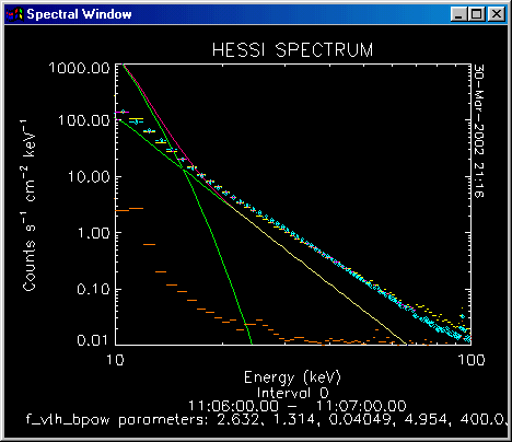
In this plot, the measured count-rate spectrum is shown as counts s-1 cm-2 keV-1 with the background added back in. Also shown are the fitted function and its components converted to count rates with background included. The difference spectrum between the measured and calculated rates is also shown.
If more than one time interval is analyzed, the power-law index can be plotted vs. time as follows:
SPEX> idl,base=getutbase()
SPEX>
idl,wset,0
SPEX> idl,utplot,avg(xselect,0),apar_arr[3,*],base
Note that "xselect" has the start and end times of the intervals that have been analyzed. For different parameters of the fits, choose the appropriate numbers for the first dimension of apar_arr
For this case, we will use a linearly varying background with different time intervals for the global energy range and for each of four user-selectable energy ranges. We first set the order of the polynomials to be used to fit the background in the different time intervals we will select by typing the following:
back_order,1,1,1,1,1
Note that the first "1" applies to the global energy range and the other four apply to each of the four user-slectable energy bins. Different background time intervals can be used for different energy bins with the parameter, use_band. The default value for use_band is -1 and this means that the background intervals apply to the global energy range. There are currently four different energy bands defined by the array ENERGY_BANDS, the same array set above for displaying the time history.
The background intervals can be set independently for the global energy range and for each of the four user-selectable energy bands (that may or may not cover the full global energy range of the selected data). We have already seen above how to select the background intervals for the global energy range by typing "background" and selecting the start and end of each interval manually. This MUST be done first with use_band set to the default value of -1. Then the background intervals are selected for each of the four energy bands in turn by issuing the following commands, where the energy band number (0, 1, 2, or 3) is substituted for i:
use_band = i
Note the equals sign instead of the comma since this is interpreted by SPEX as an IDL command and not a SPEX command.
The background intervals are then set for each energy band by typing
background
On the pop-up window, click on the "Continue by Selecting from Plot Window" button. Then move the mouse over the window with the active display ("Time History Window"). Push the left mouse button to define each side of the time intervals to be used for background determinations in that particular energy range. Note that the left edge will automatically revert to the data interval to the left of where you select; the right edge will revert to the next edge of a data interval to the right of where you select. Also, be careful that you don't click too fast. Wait after each click to see the vertical line appear on the plot and see the message appear in the IDL output log window.
Once you have selected all the intervals for background determination for that particular energy interval, move the cursor out of the Time History Window and click "DONE."
The program then computes the background as a function of time for that particular energy band and subtracts it from all the time intervals. A new time history is automatically plotted with the background subtracted.
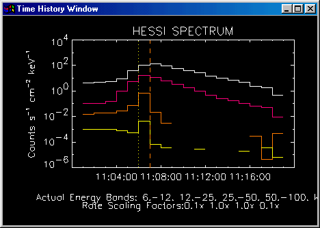
Note that I chose the first and last 1-minute intervals as background for the two lowest energy bands. For the 25 - 50 keV band, I chose intervals 3 and 9; for the 50 - 100 keV band, I chose intervals 6 and 8.
After you have selected the background and subtracted it for the global energy range and for all four energy bands, the Time History Window should look something like this:

You can now go on to select the time interval(s) for analysis as before and determine the best-fit spectra with the new background estimates.