Image Modulation Profiles

On May 3, 2010, routines to compare the expected modulation profiles from an image to the observed count rates were added to the RHESSI image object software. Previously, this comparison was plotted and some parameters stored in the Forward Fit and Pixon algorithms, but now it can be done for any image algorithm and statistics are saved for separate detectors. New info parameters containing the result of the comparison are stored in the image object, and plots can be generated to show the profiles.

These parameters and plots can be generated during and after construction of a single image using any RHESSI image algorithm (visibility-based or non-visiblity-based). However, because the calibrated event list used to make the image must be available to compute the profiles, for image cubes we have the following restrictions:

Using this tool, we've discovered that the CLEAN images often fail to match the observations when the finer detectors are included. Please see the section at the end of this page on a new Clean Regress method for computing the final CLEAN image.

Profile Plots:

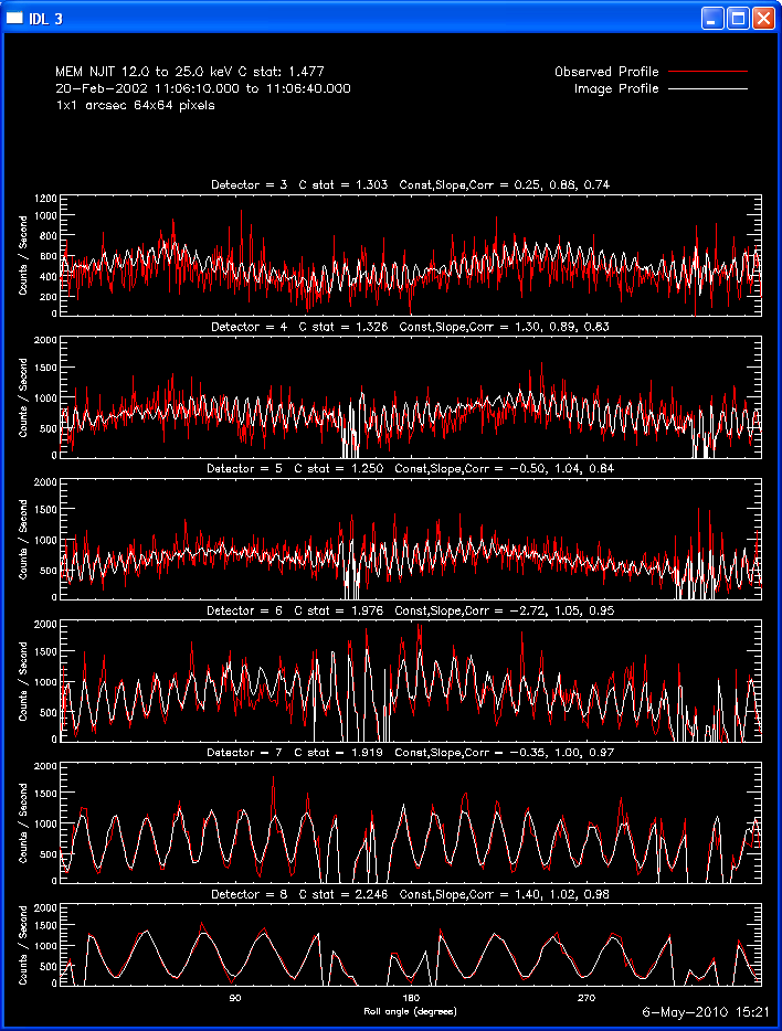
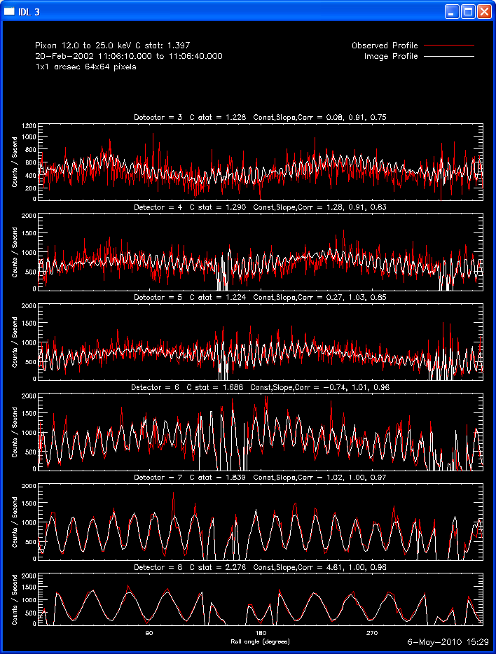
The profile plots show, for each detector selected, the observed modulation profile in red, overlaid by the expected modulation profile computed from the image in white. If the phase stacker option was enabled, the x axis is the roll angle in degrees (each detector's offset is accounted for so that in the stacked plots, the profiles for each detector are on the same x axis). If the phase stacker was not enabled, the x axis is the time of the observation in seconds relative to the start of the observation. The default plots show Counts / Second, but Counts / Bin plots can be requested. A residual plot ( (observed - expected )/ sqrt(expected) ) can also be requested.

New Info Parameters:

The following new info parameters are stored for each image for all algorithms (except vis algorithms in an image cube).

The C-statistic is computed according to Ed Schmahl's derivation from the Cash paper (ApJ, 228, 939, 1979) (using the routine hsi_pixon_gof_calc.pro) which is what Forward Fit and Pixon have been using.

Retrieve these parameters as you would any other info parameter, e.g. for a pixon image:

How to display profiles from the command line:

These image object control parameters control plotting profiles during the generation of images:

every time you generate an image, a rate profile plot will be displayed on the screen. If you also set profile_ps_plot, i.e.

then the plots will be sent to an auto-named PS file in your current working directory every time you generate an image.

To display the profile later for the most recent image generated, call the hsi_image_profile_plot routine. See the header of that routine for all keyword options. Note that options you don't explicitly specify in the keyword arguments will take their value from the corresponding parameter in the image object (i.e. if the image object parameter profile_plot_rate is set to 1, then you must call hsi_image_profile_plot with rate=0 if you don't want a rate plot). Examples (where o is your image object):

You can also retrieve the c-statistic and coefficients, and the values plotted in the profiles by providing output keyword arguments, for example:

How to display profiles from the GUI:

To display the profile plot automatically every time you generate an image, click either the 'Screen' or 'PS' box under 'Profile Plots'.

If you want to display the profiles after an image was generated, use the option in the 'Display->' button called 'Count Profile vs Roll Angle'. There are three options from that button - 'Counts / bin', 'Counts / sec', and 'Residuals', to allow you to choose what to plot. These plots are shown in a newly created plot window.

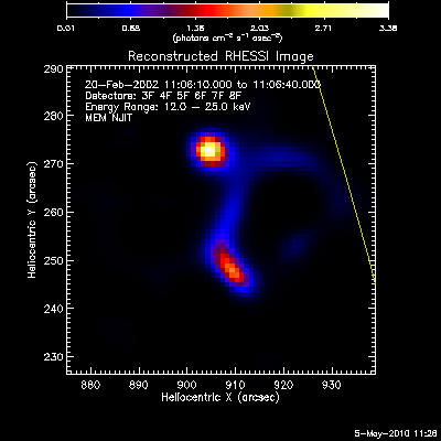
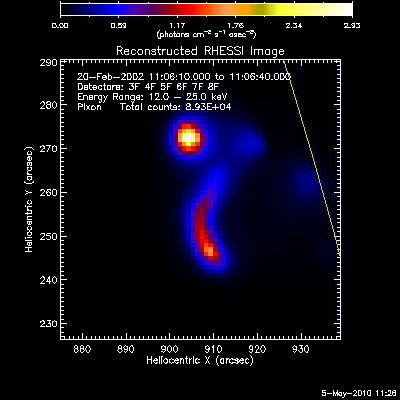
Discussion and Examples

There is one basic objective measure of the success of any image deconvolution algorithm: it should successfully reproduce the observation in a way that's consistent with the statistics of the detector measurement process. In our case, we are counting independent photon events that obey Poisson statistics. So the predicted counts should agree on average and in detail with the measurement. These image profiles help us determine this agreement at a glance. For example, if the predicted profiles are everywhere larger or smaller than the observed for all detectors then we know that there is a probably an error in the overall normalization of the image, certainly it hasn't been optimized. If there is such a discrepancy in the profile for one detector and not all then there is still a problem but one that is more subtle. Another way to evaluate the profiles is to compare the modulation depth of the predicted and observed. The image source size determines this modulation depth so an image that is too wide will show insufficient modulation depth to be consistent with the profiles in one or more of the finer grids. Finally, an exact match between the predicted and observed profiles is not a requirement or even desirable with perfect count statistics as simulation has shown that for our images it means that we will probably have degraded the true image into a collection of spurious sources.

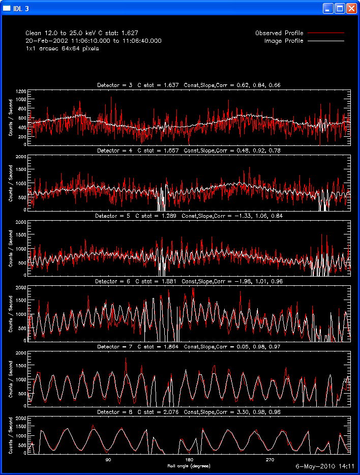
Here are some examples of the profile plot for images of the Feb-20-2002 flare using several algorithms. The time of the image is 20-Feb-2002 11:06:10.000 to 11:06:40.000, phase stacker was enabled, weighting was natural, and the flux smoothing time was 2. s.

Comments on Clean image The overall normalization appears to be good with the slope fit coefficient mostly hovering close to 1. The image appears too coarse though because of the poor match of the modulation in the finer grids. For this map, we might try increasing the clean_beam_width_factor.

Comments on UV_SMOOTH image There appears to be a mismatch in overall normalization, the predicted profiles are 10-20% larger than the observed. There is also a mismatch between the modulation profiles in Detector 3 where the predictions show less variability suggesting that the image source size should be smaller.

Comments on MEM NJIT image: We see excellent agreement on all of the grids for this image. The slope for the four coarsest grids are all close to 1.0 and we see good agreement on the finer details for all the grids. The image does not appear to be fragmented and agrees substantially with the image from Pixon.

Comments on PIXON image: While somewhat better at fitting the average and the detailed modulation, it seem as though the source sizes in the image are too broad to pick up the finer details of the time profiles in the finer grids and that there are significant deviations in some of the bins for the coarser grids.

New Clean Regress Method

We have noticed problems with the final Clean image of some flares when we've included the finer grids. The final step of the Clean algorithm as currently implemented is to add the Clean components map to the residual map to produce the final map. In certain cases, this results in final images that fail miserably on Point 1 above - the average measured and observed do not agree.

We have implemented an alternate method for combining the component and residual map that will guarantee a better match between the average observed and measured profiles. This method combines the components map with the residual map based on a regression of the count rate profiles from each of the two maps against the observed profile. (Unfortunately, mismatches caused by problems in single detectors will remain.) The new method is enabled in the objects by setting the parameter CLEAN_REGRESS_COMBINE to 1 (via a button in the Clean 'Set Parameters' widget, or o->set, /clean_regress_combine). The default value of this parameter is 0, meaning the new method is not used by default.

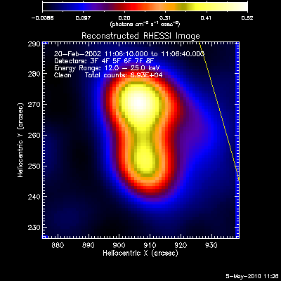
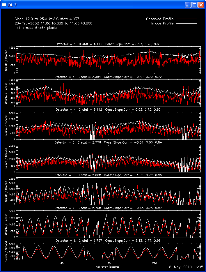
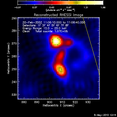
The first image and profile below shows the problematic Clean image for the same image in the example above, except that Grid 1 was included. Note the offset between the image and observed rates (this is reflected in the slopes of ~.7 - .8; a good match has a slope of 1.)

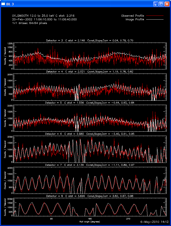
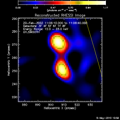
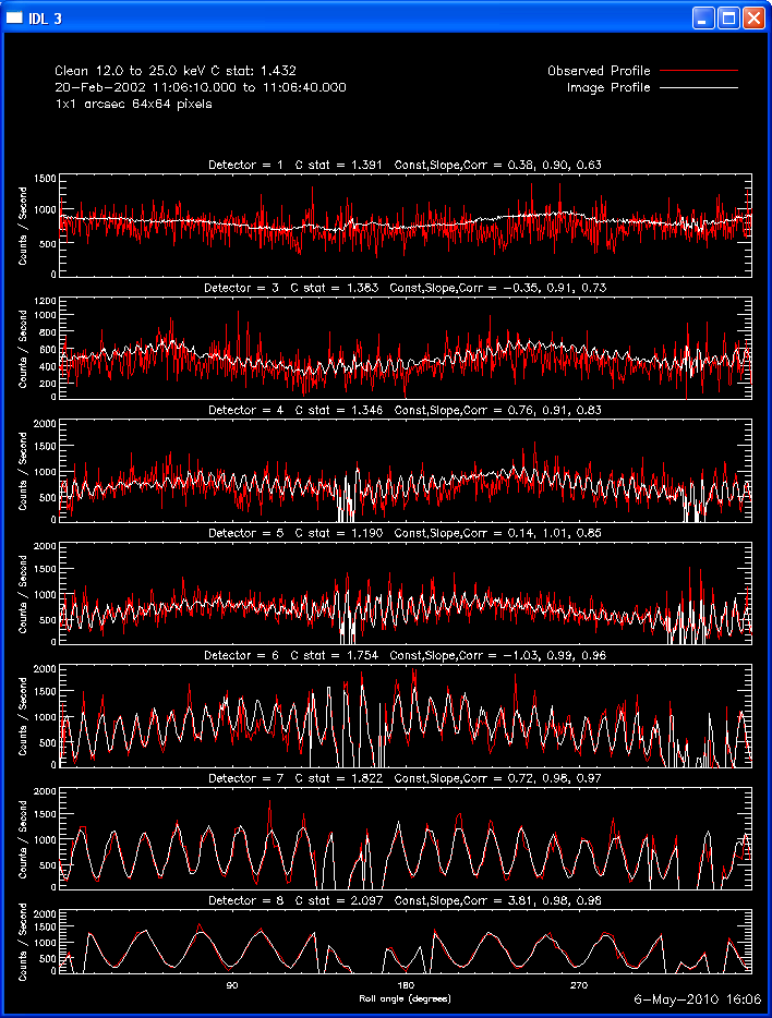
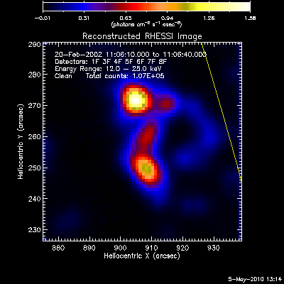
The second image and profile below show the better Clean regressed image. By using regression, we force the fluxes/profiles to match on average (note the slopes of .9 - 1.0). This also helps mitigate the effect of incomplete Cleaning where there may be a patch of flux left in the residuals. By using regression we preserve some of the inherent uncertainties from the residuals, but make the best linear combination of the two maps. Note also that the Clean Regress method does little to improve the correlation coefficient. Mismatches in source size will barely be affected by this technique.

An idea for the future: This method suggests a method for selecting the best convolving beam width to use with the point sources in the clean_source_map. We could take the component map, convolve it with a Gaussian of a given width, fit the final result using the Regress method, and then do an overall comparison for the best C statistic. Since that would probably favor overly compact source sizes, we could also add a cost function that would favor smoothness.

Name (replace 'xxx' by the prefix for the algorithm in use, e.g. 'clean')	Type	Description
xxx_profile_tot_cstat	Scalar	The overall C-statistic from the comparison of expected to observed modulation profiles for all selected detectors
xxx_profile_cstat	Array [9]	The C-statistic from the comparison of each separate detector's expected and observed modulation profile.
xxx_profile_coeff	Array [3,9]	The constant, slope, and correlation coefficient between the expected profile and observed profile for each detector. Apply the constant and slope to the expected profile to match the observed profile. Note that the constant is in units of counts / bin. The correlation coefficient gives an overall estimate of the correlation between the expected and observed profiles.

Clean image as currently implemented (clean_regress_combine = 0) Note the offset between image and observed profiles

Clean image with new regress combine method (clean_regress_combine = 1) Note the better match between image and observed profiles