OSPEX - Object Spectral Executive
OSPEX Overview
OSPEX vs SPEX
OSPEX Setup
Environment Variables
Printing
Warnings and Limitations
OSPEX Error Handling
OSPEX Batch ModeOSPEX Steps
Input Data
RHESSI Spectrum FITS, RHESSI Response Matrix FITS
RHESSI Image Cube FITS
Imaging Spectroscopy with OSPEX
'ANY' Input
User Data
Background
Fit Intervals, Options, and Fitting
Viewing Fit ResultsAdding New Data Types to OSPEX
Saving and Restoring OSPEX Session
Saving and Restoring OSPEX Results
Converting between Counts and Photons
Plotting in OSPEX
Extracting Data from OSPEXFit Function Components
Using the FIT_FUNCTION Object
Using the Nuclear Template Function
Albedo Correction
Adding User Fit FunctionsMultiple Filter (Attenuator) States
Fit Parameter Uncertainty Analysis
OSPEX Monte Carlo Analysis
OSPEX Chi-Square Mapping Analysis
OSPEX (Object Spectral Executive) is an object-oriented interface for X-ray spectral analysis of solar data. It is the next generation of SPEX (Spectral Executive) written by R. Schwartz in 1995.
Through OSPEX, the user reads and displays the input data, selects and subtracts background, selects time intervals of interest, selects a combination of photon flux model components to describe the data, and fits those components to the spectrum in each time interval selected. During the fitting process, the response matrix is used to convert the photon model to the model counts to compare with the input count data. The resulting time-ordered fit parameters are stored and can be displayed and analyzed with OSPEX. The entire OSPEX session can be saved in the form of a script and the fit results stored in the form of a FITS file.
This document is a reference manual for OSPEX. See (and contribute to) the RHESSI OSPEX User Guide wiki for detailed step-by-step instructions for using OSPEX to analyze RHESSI data in particular.
OSPEX is designed to work with any type of data that can be structured in the form of time-ordered count spectra. Usually a response matrix is needed to relate a model spectrum to the observed response. As of 2015, RHESSI, Fermi, SOXS, MESSENGER, Yohkoh, SMM, and SMART data analysis have all been implemented in OSPEX. Data types continue to be added as OSPEX evolves.
OSPEX can be run from the IDL command line or from a graphical interface, or a combination of the two. The user creates an OSPEX object at the command line and can invoke (and terminate) the main OSPEX GUI or any of the widget interfaces to subsections of OSPEX any time, or run entirely from the command line.
OSPEX is structured around a chain of objects in which each object automatically keeps track of its dependencies and knows when reprocessing is required. The lowest-level object in the chain reads data from the requested source; above that are objects for background selection, detector response information, fitting options and more; the highest level object stores and presents the fit results. This object hierarchy of OSPEX lends itself to easy expansion in both functionality and accessibility.
The OSPEX objects are built with the same framework components as the RHESSI object software. There are control parameters that you set to control the OSPEX operations, and there are info parameters that are set by the programs to record the results. The basic methods available are the same as with RHESSI objects: GET, SET, GETDATA, PLOT, PLOTMAN. The techniques for getting parameters or data from a class within OSPEX are also the same: e.g. GETDATA(class=xxx).
The OSPEX GUI is built around the PLOTMAN package and is similar to the RHESSI GUI. There are buttons under File to select OSPEX options and do fits, as well as some generic tasks like printing plots, creating plot files, and saving the OSPEX data or session. Under Plot_Control are buttons to change plotting options, zoom etc, and under Window_Control are buttons to access previously drawn plot panels. Left-clicking and dragging zooms into a plot, single left-clicking unzooms, and right-clicking displays coordinates.
OSPEX is entirely separate from SPEX. The goal is to eventually include all of SPEX's functionality in OSPEX, with the exception of some of the data types that SPEX handles.
SPEX handles a large number of instruments including: SMM (HXRBS, GRS Gamma, GRS X1, and GRS X2), Yohkoh (HXT, HXS, GRS, and SXT,) CGRO (BATSE SPEC and BATSE LAD), WIND (TGRS), HIREX, and NEAR (PIN). In principle, all of these data types can be implemented in OSPEX.
In SPEX, there were a fixed set of functions and function combinations from which to choose. In OSPEX, there are a fixed set of function components - you choose from among the components, including multiple copies of the same component, and build your own function. Also, in OSPEX, you can add your own function components.
OSPEX provides easy-to-use graphical and command-line interfaces.
To run OSPEX, you must have IDL version 5.6 or later with SSW installed. The following SSW instruments/packages must be included: HESSI, XRAY, SPEX.
OSPEX and the original SPEX are distributed together in the SSW SPEX package. In the $SSW/packages/spex/idl directory you will now see two subdirectories:
$SSW/packages/spex/idl/original_spex - contains IDL modules for the original SPEX program
$SSW/packages/spex/idl/object_spex - contains IDL modules for the new object OSPEX program
Environment variables used by OSPEX:
| SSW_OSPEX | Must point to the directory
containing the OSPEX IDL routines. Default is $SSW/packages/spex/idl/object_spex |
| OSPEX_MODELS_DIR | Must point to the directory containing the file fit_model_components.txt, which contains the list of fit function components available to OSPEX. Default is $SSW_OSPEX. |
| OSPEX_DOC | Must point to the directory
containing the OSPEX documentation. Default is $SSW/packages/spex/doc |
| OSPEX_NOINTERACTIVE | If 1, no interactive windows are
allowed. Default is 0. |
| OSPEX_DEBUG | If > 0, errors will cause normal
crashes. Otherwise errors are trapped by error handlers, and
crashes are averted. Default is 0. |
These variables are set by the file $SSW/packages/spex/setup/setup.spex_env which will be run during your SSW startup if SPEX is included in your SSW_INSTR instrument list. For most users, the default values are fine, so you do not need to take any action to set the environment variables. If the default for any of those variable is not suitable, follow the normal procedure of copying the setup.spex_env file to your $SSW/site/setup or $HOME directory and modify it. Or, from the IDL command line, you can enter something like:
set_logenv, 'OSPEX_NOINTERACTIVE', '1'
set_logenv, 'SSW_OSPEX', 'D:/my_ospex'
add_path, '$SSW_OSPEX'
Note that the OSPEX and SPEX environment variables are both set in the same setup.spex_env file.
To run the OSPEX GUI, you probably want to set up a few more environment variables:
| PSLASER | Laser printer queue Usually defined in your personal IDL startup file. |
| PSCOLOR | Color printer queue Usually defined in your personal IDL startup file |
Example:
On a Windows machine the following lines might be in your personal IDL startup file:
set_logenv, 'PSLASER', '\\kimt\laser-g62'
set_logenv, 'PSCOLOR', '\\kimt\tek-560'
Note: the printer queues must already be established on your computer. On Windows machines, the printer queues must be shared (see printing section).
The printers available for use by the OSPEX GUI are listed when you click the File / 'Select Printer...' button on the GUI. Printers are defined differently on UNIX and Windows.
UNIX
The /etc/printcap (DEC, Linux) or /etc/printers.conf (Sun) file is examined to find the list of available printers. If this file doesn't exist, then the program checks these environment variables for printer definitions:
'PRINTER', 'PSLASER', 'PSCOLOR', 'PSCOLOR2'
Windows
On Windows the program checks these environment variables for printer definitions:
'PRINTER', 'PSLASER', 'PSCOLOR', 'PSCOLOR2'
You must first set up the printers as shared and then you must define one or more of the variables listed above.
To set up printer sharing:
- On your Windows desktop, click Start, Settings, Printers.
- Right-click the printer, enable sharing, and enter a printer share name.
You should define at least PSLASER and PSCOLOR in your personal IDL startup file, by adding lines like the following:
set_logenv, 'PSLASER', '\\kimt\laser-g62'
set_logenv, 'PSCOLOR', '\\kimt\tek-560'replacing kimt with your computer name and laser-g62 and tek-560 with the share names of the printers.
-- NOTE: The following limitation no longer applies:
Currently, once you have started saving fit results, you are not allowed to change your fit time intervals or fit_function. Therefore, you should set all of your fit time intervals and all of the components of your fit function at the beginning. If you change the fit time intervals or the fit function, the spex_summ... parameters storing your results will be reinitialized, deleting your previous results. A message will warn you this is about to happen, and give you the opportunity to cancel so that you can save your previous results first. This limitation will be removed in the future.
After November 2006, if you change your fit function after you've already stored some fit results, the appropriate spex_summ... fields will be adjusted to either remove array elements or add elements to account for the change. After March, 2007, you are also allowed to change your fit time intervals after storing some fits. The spex_summ arrays will be adjusted accordingly (so the interval number may change, but the information stored will be preserved for any new interval times that match old interval times).
-- NOTE: The following limitation no longer applies:
I
f you switch to analyzing a different flare in OSPEX, it's probably safer at this point to destroy your old object (obj_destroy,o) and start a new one. Currently the parameters in the object are not reinitialized when you switch input files, so I'm not sure what will happen.
After February 2006, when you set a new input file, all of the OSPEX parameters are reinitialized.
-- We need a better way to estimate starting parameters for fits. If your parameters are too far off, the fits totally fail. Also if you are looping through time intervals using the "Previous Interval" method, once there are NaN's in the results for a fit for an interval, the rest of the intervals can't be fit. You can start at the interval that was bad, adjust its parameters, and then loop from there. Also note that there is a "Reverse" mode so that you can start fitting at the peak manually, and then loop backward and forward from there.
-- The only fitting algorithm available currently is mcurvefit. We plan to add other algorithms.
-- Separate detectors are not implemented yet.
When errors occur in OSPEX, normally they are trapped and control is returned to the main level. You may see messages about aborting and returning -1's. You should be able to continue in OSPEX. This is true for most foreseeable errors (e.g. user tried to plot data without having defined an input file). For errors that occur as a result of a bug in the code, OSPEX may crash. In this case, type retall to return to the main level. In most cases, you will be able to continue. Please report the bug to Kim Tolbert .
If you prefer not to use the trapping mechanism (so that errors will cause a crash and halt in the crashing routine), you can set the environment variable OSPEX_DEBUG to something other than 0. You can set this for new IDL sessions in your local setup.spex_env file. Or to change it in your current session of IDL, type:
spex_debug, 1
To return to error trapping mode, type:
spex_debug, 0
OSPEX can be run without any interaction required by setting the OSPEX_NOINTERACTIVE environment variable to 1. Type all of your OSPEX commands in a script (or set them up in the object from the GUI or the command line and run the writescript method), and run the script with the .RUN IDL executive command, or by calling the script as a procedure, depending on how you wrote the script.
Setting OSPEX_NOINTERACTIVE to 1 will override the individual OSPEX parameters that control output. They can also be set individually. for example:
o->set, spex_autoplot_enable=0, spex_fit_progbar=0, spex_fitcomp_plot_resid=0
To start ospex, type any of the following:
o=ospex() or ospex_proc, o Creates an OSPEX object and invokes the main OSPEX GUI
o=ospex(/no_gui) or ospex_proc, o, /no_gui Creates an OSPEX object without the main OSPEX GUI
o is now the variable holding your OSPEX object. You can now proceed to use either the command line to call the object methods, or click the buttons under 'File' in the GUI, or both, to select options and fit your data.
To help differentiate between multiple instances of OSPEX widgets, you can pass the parameter gui_label='your label' to your call to initiate ospex, e.g. o=ospex(gui_label=' April 21 analysis') , or when you bring up any of the separate widget interfaces manually (e.g. o->xfit,gui_label='Testing'). The text in gui_label will be displayed on the title bar of the widget.
Note: Even if you choose the /no_gui option, or if you exit the GUI, you can always start it by typing:
o->gui
All of the object parameters and data persist regardless of starting or exiting the GUI. The only thing you will lose by exiting the GUI is the plot panels you had created in the GUI. You can also invoke widget interfaces to subsections of OSPEX directly by calling the methods listed here.
In the OSPEX GUI, use the buttons under File to select input files, choose background time intervals if any, choose fit time intervals, fit function, and parameters, and do the fits.
From the command line, set parameters via the SET method. The control parameter names are listed in the OSPEX Standard Control Parameter Table An example of setting input files and intervals and fitting each interval to a vth+bpow function follows:
o = ospex()
o->set, spex_specfile='d:\ospex\hsi_spectrum_20020220_105002.fits'
o->set, spex_drmfile='d:\ospex\hsi_srm_20020220_105002.fits'
o -> set, spex_bk_time_interval=[['20-Feb-2002 10:56:23.040', '20-Feb-2002 10:57:02.009'], $
['20-Feb-2002 11:22:13.179', '20-Feb-2002 11:22:47.820'] ]
o->set, spex_eband=get_edge_products([3,22,43,100,240],/edges_2)
o->set, spex_fit_time_interval=[ ['20-Feb-2002 11:06:03.259', '20-Feb-2002 11:06:11.919'], $
['20-Feb-2002 11:06:11.919', '20-Feb-2002 11:06:24.909'], $
['20-Feb-2002 11:06:24.909', '20-Feb-2002 11:06:33.570'] ]
o->set, spex_erange=[19,190]
o->set, fit_function='vth+bpow'
o->set, fit_comp_param=[1.0e-005,1.,1., .5, 3., 45., 4.5]
o->set, fit_comp_free = [0,1,1, 1,1,1,1]
o->set, spex_fit_manual=0
o->set, spex_autoplot_enable=1
o->dofit, /all
More details about each step are provided below. For each step, an explanation of the widget interface is provided, followed by some command line explanations and examples.
As mentioned earlier, a combination of command line and widget clicking can be used to set parameters. On most of the widgets, there is a 'Refresh' button - use this to update the values shown in the widget if you have changed parameters at the command line.
You can view a summary of your current OSPEX parameter setup by clicking the File/Show Setup Summary button, or from the command line, typing
o->setupsummary (see the setupsummary description for print and file options)
The types of data OSPEX can handle currently (July 2016) are:
| 'ANY' | User-provided software readers for spectrum and response files | More information in the next section. |
| Fermi | GBM
CSPEC FITS files and RSP files
GBM CTIME FITS files and RSP files LAT spectrum files (PHA2) and RSP files |
Automatically downloaded for your specified time
interval by OSPEX GUI. Use gbm_find_data from command line. GBM Spectrum Archive, GBM RSP Archive, LAT Archive, Quicklook Plots, Fermi Solar Data Analysis.. |
| Konus-Wind | S1 and S2 spectrum files | Automatically downloaded for your specified time
interval by OSPEX GUI. KW data info, KW data archive, |
| MESSENGER | SAX spectrum files | Automatically downloaded for your specified time
interval by OSPEX GUI. MESSENGER Archive You need the .dat and .lbl file for the days of interest. |
| RHESSI | Spectrum FITS files and corresponding SRM FITS file
Image cube FITS file |
You must create the RHESSI spectrum and SRM files, or the RHESSI imagecube FITS file using the RHESSI software for the time interval of interest. More information in the next section. Quicklook Plots. |
| SMART | XSM spectrum files | You must supply the files. |
| SMM | HXRBS spectrum files | Automatically downloaded for your specified time
interval by OSPEX GUI. HXRBS Archive Files are event-based. |
| SOXS | CZT and SI spectrum files | Automatically downloaded for your specified time
interval by OSPEX GUI. SOXS Archive CZT and SI are in same files. |
| YOHKOH | WBS spectrum files (GRS1, GRS2, HXS data from wda... files) | You must supply the files. |
| USER | User-provided arrays of spectrum and response data inserted into OSPEX | More information in the next section. |
Create a RHESSI spectrum FITS file from a RHESSI spectrum object either in the RHESSI GUI ('Write Output File' button on the Spectra widget) or the command line (via a command similar to spectrum_obj->filewrite, /fits, /buildsrm, srmfile=srmfilename, specfile = spfilename, all_simplify=0, /create) after setting your selections for time interval, energy and time binning, detectors, etc. Normally it is best to select a time interval that includes some background, and to select finer time binning at this stage than you will actually use for fitting, so that in OSPEX you have some flexibility in defining fit intervals. Also, since you can not fit a time interval that spans a change in attenuator state, using finer time intervals minimizes the unusable data.
RHESSI Response Matrix FITS File
Since the spectrum FITS file contains data in counts, a response matrix corresponding to the spectrum file is required in order to convert to photons. The response matrix is referred to as RM, DRM (detector response matrix), or SRM (spectral response matrix) interchangeably. It is the user's responsibility to ensure that the SRM file selected corresponds to the spectrum file selected. As of July 29, 2004, the SRM file contains a response matrix for all attenuator states (called filter states in OSPEX) that occurred during the time interval of the spectrum file. OSPEX automatically uses the correct response matrix corresponding to the filter state for each time interval. SRM files created before July 29, 2004 contain a response matrix for a single attenuator state, and the user must manually instruct OSPEX to use the correct SRM file for each fit time interval.
To select the spectrum and SRM file in the GUI, browse to find your spectrum FITS file, or type the name in directly (path included). When the spectrum file was written, the name of the SRM file that was made at the same time is recorded in its header. If that file is in the same directory (and you have not renamed it), the SRM file will automatically be selected for you. This is just supposed to be helpful - you can still change to a different SRM file if necessary. Setting the filenames from the command line is described below.
Create a RHESSI Image Cube FITS file from a RHESSI image object either in the RHESSI GUI ('Write FITS File' button on the Image Widget) or the command line (via image_obj->fitswrite) after setting multiple time and/or energy bins for making images. Since the detector response was taken into account when generating the images, no SRM file is needed.
To select an image cube file in the GUI, browse to find your file, or type the name in directly (path included). After selecting an image cube file, you must select the region(s) of the image from which to extract a spectrum. The 'Select Regions' button on the 'Select Input' widget will become sensitive for image cube input. When you select the Region Selection Widget option on that button, a panel display showing all of the images in your cube will appear. By left-clicking (and dragging if you want to select multiple images) or right-clicking, a variety of options will appear in a popup widget to let you define regions and display spectra and time profiles for the current selection of regions. Another button on the OSPEX 'Select Input' widget lets you choose which region (including all regions) to use for computing spectra. The spectrum for each time interval in the image cube is the input to OSPEX. From this point, you can proceed in OSPEX as though you had started with a spectrum FITS file (with a few minor differences).
An option added 21-Feb-2006 allows you to undo the conversion from counts to photons by applying the diagonal SRM in reverse, and calculating the full SRM for a better approximation of the photon flux. This is especially important at low energies where K-escape is a significant factor, and is only taken into account in the full SRM.
More details are provided in Imaging Spectroscopy with OSPEX.
Setting the FITS filename, setting region selection parameters, and entering the Region Selection widget from the command line is described below.
In November 2014, a new way of supplying data to OSPEX was implemented to allow you to analyze any type of input data file by supplying your own software readers. This should be especially useful for new data types that haven't been explicitly implemented in OSPEX (yet), but that you would like to analyze. The idea is that you supply two routines - readers for a spectrum and response file - and tell OSPEX the base name of those readers. When you set the spectrum input file in OSPEX to a file that it doesn't recognize, it will call your reader routines. The details of the input and output required from your two routines are here.
Notes:
- This method could be used even when your data is not in a file, but is an array. The software is triggered to call the xxx_data and xxx_drm routines by encountering a file that it doesn't recognize (i.e. all of the known data types have information in the file about what kind of file they are, RHESSI, FERMI GBM, etc. which determines which reader to call.) As long as you set the spex_file_reader parameter to your routines, and set the spex_specfile parameter to any file that is not a known OSPEX data type (so any dummy file will do), your xxx_data and xxx_drm routines will be called, and you can do whatever you want in those routines, e.g. just fill the structure with data constructed by any means. This may be an easier approach than using the User Data method described below to input arbitrary data.
- If you want your data type to eventually be a 'known' data type in OSPEX, this is a good way to start - you write the reader for the spectrum and response files, and when working, pass them to us to incorporate into OSPEX.
In addition to reading data from FITS files, you may want to insert data acquired by some other means into OSPEX to fit. In order to input data directly into OSPEX, you must use the command line - there are no GUI buttons for this feature. The methods for entering data are discussed below in the Input Data from the Command Line section.
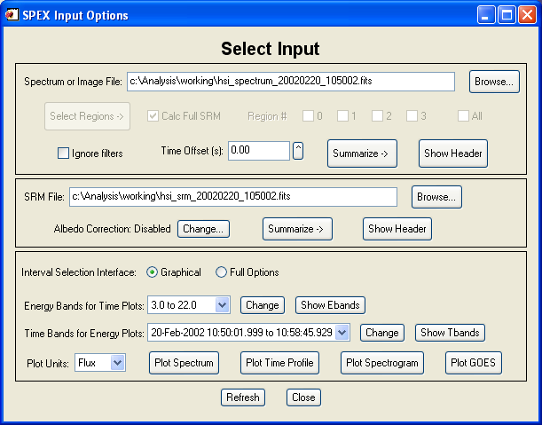
The widget interface for setting input files is invoked by clicking 'Select Input...' under File in the Main OSPEX GUI, or by typing o->xinput from the command line.
The 'Summarize' button summarizes the contents of the selected file.
In some regimes (e.g. high-energy rear detector RHESSI data analysis), you may want OSPEX to ignore the filter states. Click Ignore Filters.
The Time Offset allows you to shift the entire data array for cases where you know the time information in the file is incorrect. Note that if you have set other time intervals (background, fit) they will not be changed, but the data in those intervals is now different and will be re-accumulated.
The plot options in this window are simply for reviewing the data. Energy band selection is for selecting the energy bands that the data will be grouped into for display in time plots. Time band selection is for selecting the time bands that the data will be grouped into for display in spectrum plots. For RHESSI data, the energy bands default to the nine standard quicklook energy bands. For other types of data, the energy range is divided into 4 bands. The time bands default to 4 bands covering the time range of the file. Click the appropriate 'Change' button to change the energy or time bands. The Graphical vs Full Options buttons let you choose whether to go directly to the graphical interval selection widget for selecting bands, or to the full option interval selection widget (which includes the graphical selection widget as one of its options).
For Spectrum plots, the default is to sum all time intervals. Click 'Plot_Control' / 'XY Plot Display Options' to plot the individual time bands either summed or separately.
Note that under the SRM File selection, albedo correction information is listed, with a button to let you change the settings.
Input Data from the Command Line
Parameter Names: spex_specfile, spex_eband, spex_drmfile, spex_data_source, spex_error_use_expected, spex_ut_offset
Additional parameters available when input is an image cube: spex_image_full_srm, spex_roi_infile, spex_roi_outfile, spex_roi_use, spex_roi_integrate, spex_roi_size, spex_roi_color, spex_roi_expand, spex_ignore_filters
Spectrum FITS file Input
From the command line, to set the spectrum FITS file, DRM file, summarize the input files, set energy bands for plotting, and make some plots, use commands similar to the following:
o->set, spex_specfile='d:\ospex\hsi_spectrum_20020220_105002.fits'
o->set, spex_drmfile='d:\ospex\hsi_srm_20020220_105002.fits'
o->preview
o->set, spex_eband=get_edge_products([3,22,43,100,240],/edges_2)
o->plotman,class='spex_data', spex_units='flux', /pl_energy ; spectrum plot
o->plotman, class='spex_data', spex_units='counts' ; time profile in energy bands
To summarize all the spectrum or srm FITS files in the current directory, type:
list_sp_files (for all *spectrum*.fits files)
list_sp_files, /rm (for all *srm*.fits files)
Image Cube FITS file Input
To select a RHESSI image cube FITS file, set spex_specfile as above to your image cube FITS file. Do not set spex_drmfile. Then set the option to use the full srm if desired, the region (ROI) selection parameters (optional), and enter the ROI selection widget:
o->set,spex_specfile='d:/ospex/hsi_imagecube_2tx13e_20030723_043346.fits'
o->set, /spex_image_full_srm
o->set, spex_roi_size=100, spex_roi_color=10, spex_roi_infile='roi_2tx13e.sav'
o->roi
You can also use the widget for setting ROI options from the command line by typing:
o->roi_config
User Input
There are two methods for entering user data into OSPEX. In the simplest case, you may have an array that you want to fit using OSPEX - if you supply the spectrum array and energy edges to OSPEX, everything else will be set to default values and you can proceed to use the fitting and plotting capabilities of OSPEX. In the second case, you may want to use a RHESSI FITS file to get started, but manipulate the data or error yourself, and then insert it back into the OSPEX objects before proceeding with fitting. These two methods are discussed in detail below.
1. Using OSPEX to fit a user array
(Note: the new 'ANY' method described above for using a data type that is not 'known' to OSPEX is preferable, if you can use it.)
To set data directly into OSPEX, you must use the command line to select the 'SPEX_USER_DATA' input strategy and input your data with commands like the following:
o -> set, spex_data_source = 'SPEX_USER_DATA'
o -> set, spectrum = spectrum_array, $
spex_ct_edges = energy_edges, $
spex_ut_edges = ut_edges, $
errors = error_array, $
livetime = livetime_arraywhere
spectrum_array - the spectrum or spectra you want to fit in units of counts, dimensioned [n_energy], or [n_energy, n_time].
energy_edges - energy edges in keV of spectrum_array, dimensioned [2, n_energy].
ut_edges - time edges of spectrum_array in anytim format (if seconds, since 1/1/1979)
Only necessary if spectrum_array has a time dimension. Dimensioned [2, n_time].
error_array - error in spectrum_array in units of counts. Array must match spectrum_array dimensions. If not set, defaults to all zeros.
livetime_array - livetime in seconds. Array must match spectrum_array dimensions. If not set, defaults to all ones.You must supply at least the spectrum array and the energy edges. The other inputs are optional. By default, the DRM is set to a 1-D array dimensioned [n_energy] of 1s, the area is set to 1., and the detector is set to 'unknown'. To change them, use commands like the following:
o -> set, spex_respinfo=2. ; sets all elements of 1-D DRM (dimensioned by the same n_energy as above) to 2.
o -> set, spex_respinfo=fltarr(100,100)+.5 ; sets all elements of a 2-D DRM to .5
o -> set, spex_area=2.
o -> set, spex_detectors='mydetector'Area is in units of cm^2. Resp_info (DRM) is in units of counts/photon/keV.
Then you may continue with the widget interface, or with the command line interface.
NOTE 1: If you had selected a DRM file previously, but don't want to use it, you must set spex_drm to a null string (i.e., o->set,spex_drm='' ). If you do want to use the DRM from that file, it MUST match the data you input.
NOTE 2: The default value for spex_error_use_expected is 1, which means that the errors used in the fit are computed by combining the expected count rates with the background count rates and the systematic error, i.e. the errors on the data array are not used. If you want to use the error you set into the object (they will still be combined with the systematic error), set this parameter to 0 (i.e. o->set, spex_error_use_expected=0 )
2. Replacing data read from a FITS file
After reading data from a FITS file, you can replace the original or background data counts, error, and/or livetime in the OSPEX objects with your own data using the replacedata method. The data object (spex_data) and the background object (spex_bk) both return a structure on the getdata call that contains the following tags:
struct.data - counts data
struct.edata - error in data
struct.ltime - livetime in seconds
This method replaces any of those three structure tags in either the original (use /orig keyword) or background (use /bkdata keyword) data, and then writes the structure back into the object (via a call to setdata). Look in the object methods table for keywords to use in calling replacedata.The new counts and error arrays must be in units of counts. Fitting is done in units of rate, so even if you don't put correct livetimes into the ltime tag in the structure, you really just need to make sure that everything is consistent.
Note 1: The errors in the spex_data getdata structure are not used in computing best-fit parameters in OSPEX unless you set the spex_error_use_expected variable to 0. The default value for spex_error_use_expected is 1.
Note 2: When you replace the original data (/orig flag), the background data will be re-accumulated from the original data by default next time you do anything that retrieves the background data. (The objects for each step of data processing are set up as a chain of dependencies - when a lower element in the chain changes, everything that depends on it also changes. When none of the lower elements has changed, each object just returns the data it accumulated previously.) If you want to replace both the original and the background data, set the original data first, then the background data.
Here's an example where we read an array called spec in units of flux dimensioned to 1600 from an idl save file. The data from the FITS file is dimensioned [1600,5], i.e. 1600 energy bins, 5 time intervals. We can either rebin spec to 1600,5 and replace all of the time intervals with the same data, or we can just replace the first interval. This example does the latter, and sets the livetimes to 1. Note that since the data in the save file was in flux, we first convert it to counts by multiplying by the area and the energy bin width (we can ignore the time, since we're setting livetimes to 1).
restore,'accu2_spec.idlsave'
spec = spec * o->get(/spex_area) * o-getaxis(/ct_energy,/width)
o->replacedata, 1., /orig, /ltime, interval=0
o->replacedata, spec, /orig, /counts, interval=0
o->replacedata, sqrt(spec), /orig, /error, interval=0Here's another examples of reading data from one file, reading background from another file (in this case each file covers the same time and energy bins), subtracting them and inserting the background-subtracted data into ospex. Here the errors are set to the errors from the two files added in quadrature, and spex_error_use_expected is set to 0 so the errors inserted will be used for fitting (rather than the error on the expected counts):
o=ospex(/no_gui)
o->set,spex_specfile='110307976_counts_LIKE_MY_0.000_1800.000_bkg.fits'
bck = o->getdata()
o->set,spex_specfile='110307976_LAT_0.00_1800.00.pha'
data = o->getdata()
o -> replacedata, data.data - bck.data, /orig, /counts
o -> replacedata, sqrt(data.edata^2 + bck.edata^2), /orig, /error
o -> set, spex_error_use_expected=0
o->guiNote: You can also replace other information retrieved from the data file (look in the OSPEX Info Parameter Table for all parameters whose class is spex_data_strategy). You can use the SET command for this, e.g. to set the area and the energy edges:
o -> set, spex_area=30., spex_ct_edges=get_edges(findgen(10),/edges_2)
When you replace data or parameters in OSPEX, you should be careful that the units and dimensions are correct.
To revert back to the original data in the FITS file, call getdata with the force keyword set. Note: If you use the force keyword to retrieve the original background, both the data and the background arrays are set to their original values. (This is because the background object depends on the data object, and the /force gets passed down the object chain.)
d = o -> getdata(class='spex_data', /force)
d = o -> getdata(class='spex_bk', /force)
The widget interface for setting background options is invoked by clicking 'Select Background...' under File in the Main OSPEX GUI, or by typing o->xbk from the command line.
For image cube input, there is no need to subtract background since it is already excluded.
By default no background time intervals are defined which means no background will be subtracted. If you want to subtract background, first decide whether you want to use one set of background time intervals for all energies (the default), or define separate background time intervals for different energy bands. If you choose separate intervals for different bands, the default energy bands are the spex_eband energy bands that are used for viewing data. You can select different energy bands. There is no limit on the number of bands.
In either case, for each separate energy band (or all energies), you may select any number of background time intervals and the method (more on methods below) for computing the background in the band. For example, if you select method='1Poly' and two time intervals for the energy band 3.0-6.0 keV, then for each raw energy bin between 3.0 and 6.0 keV, a time profile is computed by fitting the points in the time intervals selected for that energy to a first order polynomial.
Note: the following rules are followed in nonstandard cases:
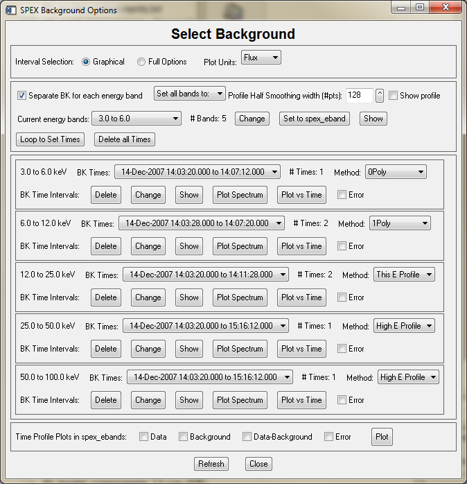
The first example below shows the widget with the separate option disabled, the second with the separate option enabled.
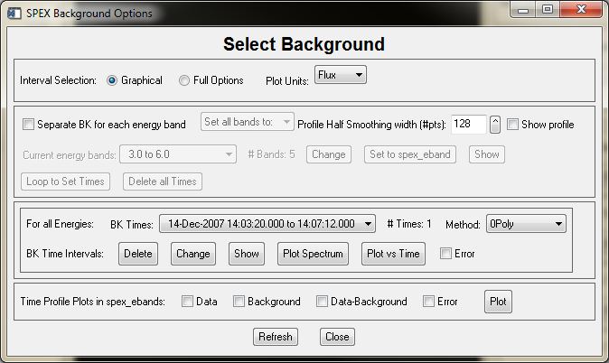
The Graphical vs Full Options buttons let you choose the graphical interval selection widget directly, or the full options interval selection widget (which includes the graphical selection widget as one of its options). This applies to both the selection of energy bands and time intervals. The selection of Plot Units applies to all plots that are available from this widget.
If separate energy bands are selected, there is a pulll-down button to easily set all the bands to the same method.
The Profile Half Smoothing width is used in the two profile methods (discussed below) to smooth the final profile. If you enable the show profile option, when the profile is computed a plot will be displayed showing the various steps in computing the final smoothed profile.
If you have not selected the separate background energy band option, then there will be one sub-widget for changing, showing and plotting time intervals and selecting the method. If you have selected the separate option, that sub-widget will expand into multiple sub-widgets, one for each energy band (it will become scrollable if there are too many energy bands to show). There is a 'Loop to Set Times' button that will automatically enter the interval selection widget (graphical or full according to your selection) for each energy band in turn. Or you can click the Change button for any individual energy band. You can also set the method individually for each energy band.
The Delete button deletes the time intervals for that energy band. Change lets you select time intervals. The Show button plots the data in the units selected, grouped in the energy bands defined by spex_eband (not spex_bk_eband, the background energy edges) and shows the time intervals selected. Plot Spectrum plots the spectrum in each time interval selected to define background for that band. Plot vs Time plots the data, the computed background, and the data minus the background for that energy band.
The Time Profile Plot options plot the options selected (data, background, and/or data minus background) grouped into spex_eband energy bands in the units selected (remember spex_eband may be different from spex_bk_eband).
The methods available for computing the background are:
0Poly - 0th order polynomial
1Poly - 1st order polynomial
2Poly - 2nd order polynomial
3Poly - 3rd order polynomial
Exp - exponential
High E Profile - use the ratio to the profile in the highest energy band
This E Profile - use the ratio to the profile in this energy band
In the five function methods (polynomials and exponential), for each raw energy bin, the background is computed by fitting the data in the time interval(s) selected to the function selected. The error is the square root of the counts used in that fit. When combining time bins, these errors are averaged.
In the two profile options, you select time interval(s) for the highest energy band (High E Profile), or the selected band (This E Profile) that include the shape you want to use. This shape is then used for each raw energy interval (scaled by the ratio of the data in the raw energy bin to the profile). More specifically,
First a smoothed interpolated profile is computed as follows:
Bin the data (in rate space) into the energy band selected
Smooth that binned data in the selected time intervals with a boxcar of width 10 (so that the endpoints we use for interpolation are good)
Interpolate across gaps between specified intervals
Smooth again using Savitzky-Golay smoothing filter
of width defined by Profile Half Smoothing width parameter.
For each data energy bin (the raw bins, not the broader energy bands you've selected), the data in the time intervals selected for the energy band containing this bin are averaged and divided by the average of the smoothed profile in those times.
The background time profile for this energy bin is computed by multiplying the smoothed profile by that ratio.
The errors on the background is the square root of the counts in the time interval(s) used to calculate the ratio. When combining time bins, these errors are averaged.
Prior to September 2013, we used a parameter called spex_bk_ratio to turn the 'High E Profile' method on for all energy bands. There was no option to select other methods for some energy bands. The spex_bk_ratio parameter still exists for backward compatibility. If you have an old script that sets it, now the method for each separate band is set to 'High E Profile'.
Background from the Command Line
Parameter Names: spex_bk_sep, spex_bk_eband, spex_bk_order, spex_bk_time_interval, spex_bk_ratio, spex_bk_sm_width.
For backward compatibility, the spex_bk_order parameter is used for the any of the six background methods, it is not limited to the order of the polynomial. The values for spex_bk_order are: 0 = 0Poly, 1 = 1Poly, 2 = 2Poly, 3 = 3Poly, 4 = Exp, 5 = High E Profile, 6 = This E Profile
Example without separate background energy bands:
In this case, spex_bk_order is a scalar, and spex_bk_time_interval is an array of n time intervals dimensioned [2,n].
o -> set, spex_bk_sep = 0
o -> set, spex_bk_order=1
o -> set, spex_bk_time_interval=[['20-Feb-2002 10:56:23.040', '20-Feb-2002 10:57:02.009'], $
['20-Feb-2002 11:22:13.179', '20-Feb-2002 11:22:47.820'] ]o -> plotman, class='spex_bkint', spex_units='flux' ; plot bk spectra in time intervals selected
o -> plot_time, /data, /bksub, /bkdata ; plot data, bksub, and bkdata in spex_eband energy bands in counts
Example with separate background energy bands:
In this case, spex_bk_order is an array dimensioned to the number of bands, and spex_bk_time_interval is a pointer array (dimensioned to the number of bands) where each pointer points to an array of n time intervals dimensioned [2,n], where n can be different for each band.
spex_bk_order can easily be set in a single call, e.g. o->set, spex_bk_order=[1,1,2], but to set spex_bk_time_interval in a single call, you must set up the pointer array and its contents yourself. For this reason, the SET and GET methods have these additional keywords to make things easier:
- this_band - The band you want to set or get data for (starts at 0)
- this_time - In call to GET, use /this_time to return the bk time intervals for this_band, e.g. time2 = o->get(/this_time, this_band=2). In call to SET, use this_time=xxx to set the bk time intervals for this_band, e.g. o -> set, this_band=2, this_time=t
- this_order - In call to GET, use /this_order to return the bk order for this_band, e.g. order2 = o->get(/this_order, this_band=2). In call to SET, use this_order=x to set the bk order for this_band, e.g. o -> set, this_band=2, this_order=3
o -> set, spex_bk_sep = 1
o -> set, spex_bk_eband = get_edges([3.,6.,11.,39.,250.], /edges_2)
o -> set, spex_bk_order=[1,1,1,2] or
o -> set, this_band=0, this_order=1
o -> set, this_band=1, this_order=1
etc. for all bands
o -> set, this_band = 0, this_time = [['20-Feb-2002 10:56:23.040', '20-Feb-2002 10:57:02.009'], $
['20-Feb-2002 11:22:13.179', '20-Feb-2002 11:22:47.820'] ]
o -> set, this_band = 1, this_time = [['20-Feb-2002 10:51:02.619', '20-Feb-2002 10:54:57.439'], $
['20-Feb-2002 11:22:33.179', '20-Feb-2002 11:22:47.820'] ]
etc. for all bandstimes0 = o -> get(this_band=0, /this_time) ; to get bk time interval for spex_bk_eband # 0
times1 = o -> get(this_band=1, /this_time) ; to get bk time interval for spex_bk_eband # 1
order1 = o -> get(this_band=1, /this_order) ; to get bk order for spex_bk_eband #1o -> plotman, class='spex_bkint', spex_units='flux', this_band=2 ; plot bk spectra in time intervals selected for band #2
o -> plot_time, /data, /bksub, /bkdata, /bkint, this_band=2 ; show data, bksub, bkdata in spex_bk_eband # 2 vs time in counts
o -> plot_time, /data, /bksub, /bkdata, this_band=2 ; show data, bksub, bkdata in spex_eband # 2 vs time in counts
o -> plot_time, /bksub, /bkdata, spex_units='flux' ; plot bksub and bkdata in flux units for all spex_eband bands vs timeTo change the background data manually, you can use the replacedata method described in the Replacing data read from a FITS file section. For example, if you want to double the existing background:
b = o -> getdata(class='spex_bk')
o -> replacedata, b.data*2, /bkdata, /counts
The widget interface for setting fit options is invoked by clicking 'Select Fit Options and Do Fit...' under File in the Main OSPEX GUI, or by typing o->xfit from the command line.
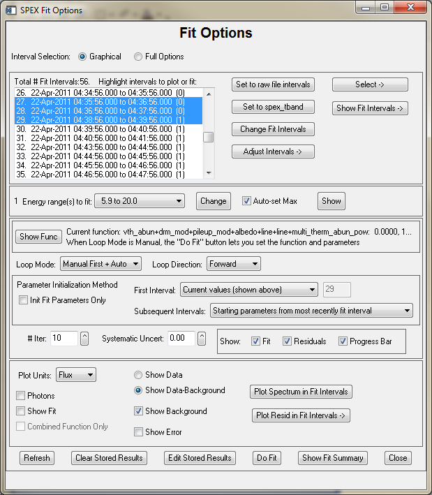
The Graphical vs Full Options buttons let you choose whether to go directly to the graphical interval selection widget, or to the full option interval selection widget (which includes the graphical selection widget as one of its options). This applies both to specifying the Fit Time Intervals via the 'Change Fit Intervals' button and selecting the Energy ranges to fit via its 'Change' button. The 'Set to raw file intervals' button sets the Fit time intervals to all of the time intervals from the spectrum file. After defining some fit time intervals, you may want to adjust them slightly. Clicking on the 'Adjust Intervals' button will give you several options (note that any of these options will also remove any intervals that contain no data) as follows:
If you see a number in parentheses after the time interval that is the filter state for the interval. These won't be shown when they are the same for all intervals. In the case above, the earlier intervals are in filter state 0, and the later intervals are in filter state 1 (since the data are from RHESSI, the filter states correspond to attenuator states 0 and 1).
The energy range to fit is shown in the widget as a pulldown menu for viewing reasons only. Usually you will have a single energy range, but it's possible to exclude parts of the spectrum by setting multiple energy ranges. The pulldown lets you see the multiple ranges, but has nothing to do with selection. By clicking the Change button you can edit the energy range(s) graphically or by text editing. When the Auto-set Max button is set, the software automatically sets the upper limit of the energies to fit based on the background-subtracted counts/bin. For energies > 10. keV, it finds the energy bin where the rate becomes less than a threshold (controlled by spex_fit_auto_emax_thresh parameter, which defaults to 10. counts/bin), and set the spex_erange upper limit to the lower edge of the bin. (Prior to 30-Oct-2013, we used the count rate > .01 counts/sec test, and rounded the energy up to the next higher multiple of 10.) You can also have the software automatically set the lower limit for the energy range to fit for RHESSI data only - in attenuator state A0, the lower limits is 4. keV, and in attenuator states A1 or A3, the lower limit is 6. keV. These features allow you to loop through intervals automatically without having to manually set appropriate fit energy ranges as the spectrum changes through the flare.
Once you have defined fit time intervals the 'Plot Spectrum in Fit Intervals' button will work. You can select single intervals or a combination of intervals to plot by highlighting the intervals or by using the options in the 'Select' button. All of the options for plotting should work at this point.
NOTE: Once you have fit an interval, the best-fit parameters will be used when you select a Photon plot and /or select the 'Show Fit' option. However, if you have not done a fit on an interval, the current function and parameter values are used. Those values will depend on what you did last and could be completely wrong for the interval you're plotting. (Notice the label on the plot saying 'No fit done'.) The photon plot will probably be meaningless! See below for more information on plotting photons.
The current function and parameter values are listed (in this case a variable thermal plus a broken power law). You must set the Loop Mode to one of the manual choices ('Manual First + Auto' or 'Manual All Intervals') in order to change the function and/or the parameters. "Manual First + Auto" enters the interactive Fit Component widget for the first interval you have highlighted, but proceeds automatically though the rest of the highlighted intervals. In automatic mode, it will automatically loop through each selected interval (those highlighted in the list of intervals).
NOTE: There are two distinct areas for storing fit parameters and results - one that is currently in use and changes every time a fit is made, and one that is a repository for storing and accumulating your fit results. The current fit function and fit parameters are stored in control parameters called fit_function, and the parameters prefixed by 'fit_comp' (fit_comp_param, fit_comp_minima, etc). You can set these parameters from the command line or through the Fit Function Component widget (discussed below). The parameters computed as the best fit parameters are also stored in fit_comp_param after a fit. However, once the fit for an interval has been 'accepted' (in the Fit Function Component widget) or when automatic looping is selected, the fit results are stored in the info parameters with the 'spex_summ' prefix. Look in the OSPEX Info Parameter Table for all of the parameters with the spex_summ prefix. When the first fit is accepted (whichever interval it is, not necessarily the first), the spex_summ variables are dimensioned according to the total number of fit time intervals, energy bands, and fit function parameters. Previously (prior to March 2008 for time intervals, and prior to November 2006 for fit function) you were not allowed to change fit time intervals or fit function after you had started saving fit results. Now, if you change either, the spex_summ... parameters are adjusted accordingly. You will be prompted to allow the changes if you are running interactively, otherwise, the changes will be made automatically. You can not change the number of energy bands.
There are two parameter initialization methods, one for the first interval in the series of intervals selected for fitting, and one for subsequent intervals in the series.
Notes: If the 'Init Fit Parameters Only' box is checked, then for each of the methods below, only the fit parameters are set from the various sources, not the minima, maxima, free mask, etc. Any values that are not set are left at their current values (the values stored in the fit_comp... parameters), which are fluid and depend on what you did last.
If 'Init Fit Parameters Only' is not selected, there are two groups of parameters that might be set depending on the initialization method:
| Group A | Group B |
| fit_comp_params | erange (note exception below) |
| fit_comp_minima | uncertainty |
| fit_comp_maxima | # iterations |
| fit_comp_free_mask | |
| fit_comp_spectrum | |
| fit_comp_model |
First interval parameter initialization methods have the meaning shown in the following table. The corresponding value of the parameter spex_fit_firstint_method is shown in parentheses (i.e. to select the method 'Final Fit Parameters from Interval n' using interval 3 from the command line, you would type o->set,spex_fit_firstint_method='f3').
| Program Defaults (default) | Group A parameter values are taken from the defaults routines for the function components in the current fit_function |
| Current (current) | Leave all the group A and B values at their current setting |
| Final Fit Parameters from Interval n (fn) |
Group A and B parameters are set as they were for interval n. The fit_comp_params values are the final fitted values from interval n. |
| Starting Fit Parameters from Interval n (sn) |
Group A and B parameters are set as they were for interval n. The fit_comp_params values are the starting values from interval n. |
Subsequent interval parameter initialization methods have the meaning shown in the following table. The corresponding value of the parameter spex_fit_start_method is shown in parentheses.
| Program Defaults (default) | Group A parameter values are taken from the program defaults for the current fit_function . |
| Fitted Parameters from Most Recently Fit Interval (previous_int) |
Group A and B parameters values from the most recently fit interval are used (e.g., if you are fitting intervals 3,6,9 in reverse order, interval 6 will get its values from interval 9.) fit_comp_params values are the final fitted values from that interval. |
| Starting Parameters from Most Recently Fit Interval (previous_start) | Group A and B parameters values from the most recently fit interval are used (e.g., if you are fitting intervals 3,6,9 in reverse order, interval 6 will get its values from interval 9.) fit_comp_params values are the starting values from that interval. |
| Fitted Parameters from Previous Iteration on each Interval (previous_iter) |
If this interval has been fit already, the
stored values of Group A and B parameters from that previous
iteration (stored in the spex_summ structure) are used.
fit_comp_params values are the final fitted values from the
previous iteration. Note: this method applies to the first interval being fit as well as subsequent intervals and overrides the 'spex_fit_firstint_method' that is set. |
NOTE - Exception for erange: If spex_fit_auto_erange or spex_fit_auto_emin is set, that adjustment to the lower or upper limit of the energy range to fit is applied AFTER the spex_erange is set based on the parameter initialization method. When in the GUI, and initialization method is Previous Iteration, you will be asked if you're sure that you want to adjust the limits. In all other cases, the adjustment will be made.
The # Iter widget sets the maximum number of iterations performed while fitting. The Systematic Uncert. widget sets the value of the systematic uncertainty. The systematic uncertainty is added in quadrature to the poisson statistical uncertainty for each data point to compute the error bar on each point. The value used for the systematic uncertainty is arbitrary - it is really a fudge factor that allows you to prevent the ridiculously small statistical uncertainties that might result from very high count rates from skewing the fit results.
The Show: Fit, Residuals, Progress Bar buttons let you select what will be displayed as we're looping through each interval. For each interval, 'Fit' will plot the spectrum and model function(s) using the options you have selected in the widget (units, photons, show bk), 'Residuals' will plot the residuals for the fit in a separate plotman window (you might want to position this below the main GUI to line them up before automatically looping), and 'Progress Bar' will display a progress bar showing you which interval it's working on, and a Cancel button to let you cancel the loop.
The Edit Stored Results button brings up a table widget that lets you easily modify some of the spex_summ values that will be used as starting points or controls (e.g. energy range to fit) for fitting, e.g. changing a parameter from fixed to free for all intervals. When you change any values for an interval, the chi-square value for that interval is set to 0. as an indication that the fit was not done with the current parameters. This table widget can be invoked from the command line via the xedit_summ method.
When you press the Do Fit button, if Loop Mode is automatic, it will automatically loop through the intervals you have highlighted. If Loop Mode is either of the Manual options, the Fit Function Components widget below will appear.
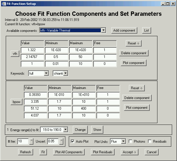
This widget lets you combine function components to construct your own function. The List button (and the button showing the name of each component) summarizes the function components that are available and the meaning of the parameters. Select a component from the droplist and click Add Component to add it. If you want two of a component, you can add another one. When the list of components gets long, the component section of the widget will become scrollable.
Note that near the top of the widget it lists which interval we're working on. You can change parameters and plot components separately or combined to see how the model compares to the spectrum for that interval. If the 'Auto Plot' option is selected, every time you change a value (and hit return so it knows you did something), the component will be plotted according to the options selected (units, photons). You can change the energy range, # iterations, and uncertainty for each interval. Once you're happy with your starting parameters, you can click Fit to see the results. If they're not acceptable, you can change parameter values and try again any number of times. There are several options for exiting this widget:
Note: although the graphical energy range selection is often convenient, that option is not available here because of widget restrictions. The Change button will pop up an editable text window. The graphical selection option is only available from the 'Fit Options' widget.
If you cancel (either by clicking Cancel in the Fit Function Component widget, or by clicking cancel on the progress bar), the intervals that have been completed so far are still saved.
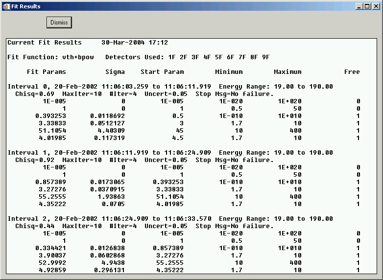
Use the 'Show Fit Summary' button to show a text summary of the fit results for each interval. For this example, it shows the following:
Fitting from the Command Line
Parameter Names: spex_fit_time_interval, spex_fit_time_used, spex_erange, spex_fit_auto_erange, spex_fit_auto_emax_thresh, spex_fit_auto_emin, fit_function, fit_comp_param, fit_comp_free_mask, fit_comp_mimima, fit_comp_maxima, spex_fit_manual, spex_fit_reverse, spex_fit_start_method, spex_autoplot_enable, spex_fitcomp_plot_resid, spex_fit_progbar, spex_intervals_tofit, spex_fit_init_params_only
Examples of commands to set these options are:
o->set, spex_fit_time_interval=[ ['20-Feb-2002 11:06:03.259', '20-Feb-2002 11:06:11.919'], $
['20-Feb-2002 11:06:11.919', '20-Feb-2002 11:06:24.909'], $
['20-Feb-2002 11:06:24.909', '20-Feb-2002 11:06:33.570'] ]
o->adjust_intervals
(o->get(/obj,class='spex_fitint')) -> find_bad_intervals,/remove
o->set, spex_erange=[19,190]
o->set, fit_function='vth+bpow'
o->set, fit_comp_param=[1., 1., 1., .5, 3., 45., 4.5]
o->set, fit_comp_free = [1,1,0, 1,1,1,1]
o->set, fit_comp_spectrum=['full', '']
o->set, fit_comp_model=['chianti', '']
o->set, spex_fit_reverse=0, spex_fit_start_method='previous_int'
o->set, spex_fit_manual=1, spex_autoplot_enable=1, spex_fitcomp_plot_resid=1, spex_fit_progbar=1
o->dofit, /all ; this will bring up the xfit_comp widget since spex_fit_manual=1Or, if you don't want to interact with the xfit_comp widget, and don't want to see plots or the progress bar, change the last two lines to this:
o->set, spex_fit_manual=0, spex_autoplot_enable=0, spex_fitcomp_plot_resid=0, spex_fit_progbar=0
o->dofit, /allAnd if you don't want to even see the little widget that says 'Fitting...' to show that it's working, set
set_logenv, 'OSPEX_NOINTERACTIVE', '1'
If you don't want to fit all intervals, select a subset by setting the spex_intervals_tofit parameters:
o->set, spex_intervals_tofit=[0,1,3]
o -> dofitThe fit time intervals you set are stored in spex_fit_time_interval. The intervals actually used are stored in spex_fit_time_used. These will be the same if you called adjust_intervals, and find_bad_intervals,/remove.
The results of the fits for all intervals selected are accumulated in the spex_summ... info parameters. The fit parameter correlation matrix showing the dependencies between fit parameters is available for the most recent fit (it's not stored in the spex_summ structure). The correlation coefficient is zero if two fit parameters are uncorrelated, 1 if they are linearly correlated, and -1 if they are linearly anti-correlated. The matrix can be retrieved by typing
print, o -> get(/mcurvefit_corr)
Note: o->dofit and d=o->getdata(class='spex_fit') both start the fitting process. d will be a structure containing the results of the most recent interval fit. In either case the spex_summ... parameters will contain the results of the fits for all intervals that have been fit so far.
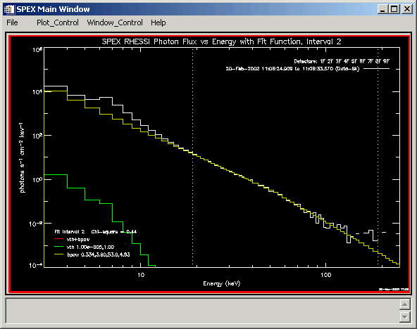
To plot the spectrum for selected intervals, showing the fit, use commands like:
o->plot_spectrum, this_interval=0, /show_fit, /use_fitted
o->plot_spectrum, this_interval=2, /show_fit, /use_fitted, spex_units='flux', /bksub, /photonThis last plot command resulted in the following plot in this example. Normally the combined function would be plotted in red, but in this case the yellow bpow function plotted separately lies on top of the combined function. The dotted lines show the energy range that was used in the fit.
To see a summary of the fit results, type:
o->fitsummary (see the fitsummary description for print and file options)
To retrieve the fit results in a structure, type:
s = o->get(/spex_summ)
Refer to the spex_summ... parameters in the OSPEX Info Parameter Table for the meaning of each element of the structure.
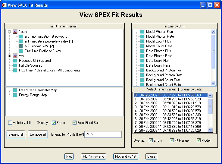
The widget interface for looking at the fit results is invoked by clicking 'View Fit Results...' under File in the Main OSPEX GUI, or by typing o->xfitview from the command line.
Viewing Fit Results from the Command Line
From the command line, you can retrieve all of the fit summary parameters (all parameters starting with 'spex_summ') via the command:
s = o -> get(/spex_summ)
Or, if the object doesn't exist anymore, you can restore the fit results from a file (FITS or geny save file) via spex_read_fit_results as described in Saving and Restoring OSPEX Results, for example:
s = spex_read_fit_results('ospex_results.fits')
Either way, s will be a structure containing everything that was saved during the fitting process, including the fit time intervals, energy edges, fit function, and for each fit interval the fit parameters, starting parameters, chisq, conversion factors, model, count rate and errors, background and errors, residuals, and more. Refer to the spex_summ... parameters in the OSPEX Info Parameter Table for the meaning of each parameter.
Note that with this structure, you should either have directly, or be able to compute all of the following: the data and background count or photon spectrum in any units, and the model count or photon spectrum in any units, i.e. the count rate spectrum, the conversion factors, and the photon model flux are stored for each time interval, and the rest can be calculated from them.
Now that you have the data, you can plot and calculate quantities from the fit results using object methods if the OSPEX object still exists, or manually if not.
1.) If you still have the OSPEX object that computed these results, you can use the plot_summ and calc_summ methods. In the first example below, we plot fit parameter 4 vs time; in the second we plot the residuals vs energy for intervals 0, 1, and 2:
o -> plot_summ, xplot='time', yplot='param', yindex=4
o -> plot_summ, xplot='energy', yplot='resid', this_interval=[0,1,2]
In the following example, we calculate the data photon flux and the photon flux errors for intervals 1 and 2:
ph_flux = o -> calc_summ(item='data_photon_flux', this_interval=[1,2], errors=data_photon_flux_errors)
The calc_summ item keyword can be set to any of a number of values - see the list below in the calc_summ description.
2.) Alternatively, you can plot and compute quantities manually. In the first example below, we plot fit parameter 4 vs time; in the second we plot the residuals vs energy for intervals 0, 1, and 2:
mid_times = get_edges(s.spex_summ_time_interval, /mean)
utplot, anytim(mid_times, /ex), s.spex_summ_params[4,*]
mid_energies = get_edges(s.spex_summ_energy,/mean)
plot, mid_energies, s.spex_summ_resid[*,0], /xlog
oplot, mid_energies, s.spex_summ_resid[*,1]
oplot, mid_energies, s.spex_summ_resid[*,2]
You can calculate the following quantities, among others:
data count flux = data count rate / area / energy width
data photon flux = data count flux / conversion factors
model count flux = model photon flux * conversion factors
For example, to compute the data photon flux (assuming s contains the spex_summ structure):
conv_fact = s.spex_summ_conv
area = s.spex_summ_area
ewidth = get_edges(s.spex_summ_energy,/width)
ct_flux = s.spex_summ_ct_rate / area / rebin(ewidth, size(s.spex_summ_ct_rate, /dim))
ph_flux = ct_flux / conv_fact
The writescript method saves an OSPEX session. Internally, there are two steps to saving an OSPEX session:
In the OSPEX GUI, use the buttons under File to 'Write Script'. Additional buttons let you choose whether to write a fit results file as well as the script file. A widget will appear to allow you to choose the names for the script file and the fit results file. The name of the procedure will be the name of the script file you select.
At the command line, type (see the writescript description for calling arguments):
o -> writescript
To run the script to restore the session, type
script_name, obj=obj
If obj is an existing OSPEX object, then the procedure will set the parameters in that object to the values they had when you wrote the script (Note - parameters not mentioned in the script will be unchanged, they will not be initialized). If not, the procedure will create a new OSPEX object and set the parameters/values. Depending on how you wrote the script, it may start the GUI, and and it may restore the fit results.
In addition, there is a button on the GUI under File to 'Set Parameters from Script' to allow you to set parameters in an existing object according to the script file (either initializing all parameters to defaults first or not). At the command line, type:
o->runscript or o->runscript, /init
If o is an existing object, then script_name,obj=o is equivalent to o->runscript.
The fit results are saved via the OSPEX savefit method which writes all of the fit results parameters (all info parameters starting with spex_summ) into a file. They are restored into the OSPEX object via the restorefit method which reads the file and uses the SET method to set the spex_summ parameters into the object. They are restored to your IDL session via the spex_read_fit_results routine.
Two types of output file are supported:
In the OSPEX GUI, use the buttons under File to 'Save Fit Results' and 'Import Fit Results'.
At the command line, type the following to save the fit results or restore fit results into the OSPEX object:
o -> savefit
o -> restorefit
Note that it is possible to include restoring the fit results as part of a script that restores an OSPEX session (see section on Saving and Restoring OSPEX Session)
To restore the fit results structure directly (without creating an OSPEX object) from either a FITS or geny file, use the spex_read_fit_results procedure. For example,
fit_results = spex_read_fit_results('ospex_results.fits')
(Geny files can also be read in directly using the restgenx command: restgenx, file='ospex_results.geny', fit_results )
The structure containing all of the fit results will be returned in the fit_results variable. Look at the parameters starting with spex_summ in the OSPEX Info Parameter Table for the meaning of each tag in the structure.
The input data (at least from a RHESSI spectrum FITS file) is in counts. The fit functions (model) calculate photon flux. Whenever you plot the data in photons, or the model in counts, a conversion between counts and photons is being calculated.
The efficiency factors (or conversion factors) used to convert counts to photons depends on both the response matrix and a model. The efficiency factors are the ratio of the model count spectrum, which is the model photon spectrum folded through the detector response, to the model photon spectrum.
Converting from photons to counts is achieved through a matrix multiplication of the response matrix with the photon spectrum.
NB: Beware of misinterpreting the photon spectrum. If the model is not a close fit to the data, or you apply the wrong response matrix, then the efficiency factors and therefore the photon spectrum, are meaningless. Similarly if you apply the wrong response matrix to the model to convert to counts, it is meaningless. That's why this is an iterative process -successive iterations in the fit process bring the model closer to the data.
The GUI has options to plot data and overlay fit functions in either counts or photons.
Getting conversion factors for converting counts to photons
If you've already analyzed and saved fits, the conversion factors are stored in the spex_summ structure:
conv = o -> get(/spex_summ_conv)
or
s = o -> get(/spex_summ)
conv = s.spex_summ_conv
The more general way to get the conversion factors (whether you've saved the fits or not) use the get_drm_eff method. With no arguments, this function uses the SRM for the current interval (in spex_interval_index) , and if available, the computed saved fit results. If unavailable, or the keyword use_fitted is set to 0, the current values of the fit function and the fit parameters (in fit_function and fit_comp_params) are used to compute the diagonals. Use the this_interval keyword to specify the intervals you want the conversion factors for.
For example, to convert data from the 5th fit interval to photons, we do the following:
d = o -> getdata (class='spex_fitint')
data = d.data[*,5]
conv = o -> get_drm_eff(this_interval=[5], use_fitted=0) ;don't use saved fit results (use current fit_comp_params values)
or
conv = o -> get_drm_eff (this_interval=[5], /use_fitted) ; use saved fit resultsspex_apply_eff, data, conv
'data' is now in photons. Note: all spex_apply_eff does is divide data by conv. Also note that to get photon rate or photon flux rather than photon counts, do the getdata above with spex_units='rate' or 'flux'.
Converting the model from photons to counts
There are several ways to do this:
1. Calculate the model in the photon energy bins. Apply the drm to get the count rate. Divide by area and energy bin width for get count flux.
ph_ener = o -> getaxis(/ph_energy, /edges_2)
params = o -> get(/spex_summ_params) ; or from fit_comp_params
phot_flux = f_1pow(ph_ener, params[0:2,2]) + f_vth(ph_ener, params[3:5,2]) ; for interval 2
drm = o -> getdata(class='spex_drm') ; if multiple filter (attenuator) states, use this_filter keyword to get correct drm
count_rate = drm # phot_flux ; returns count rate
count_flux = count_rate / o->get(/spex_area) / o->getaxis(/ct_energy,/width)
2. Use the calc_func_components method. This is the easiest and most flexible.
count_flux = o -> calc_func_components(this_interval=2, /use_fitted, photons=0, spex_units='flux')
The calc_func_components returns a structure with the spectrum for the combined and separate model components in photons or counts, in units of counts, rate or flux for the interval(s) specified. See the calc_func_components explanation below for details.
3. If you haven't saved the fits yet, you might want to use this method. Get the model data in photon flux from the fit_function object and use the convert_fitfunc_units method to convert to counts. For example,
model_ph_flux = o -> getdata(class='fit_function') ; the model will be calculated using the current fit_comp_param values
model_count_flux = o -> convert_fitfunc_units (model_ph_flux, photons=0, use_fitted=0, $
spex_units='flux', this_interval=2) ; interval # is needed to use correct drm (in case where there are multiple filter states)
or use spex_units='rate' to get the model_count_rate.
Most of the object classes have plot and plotman methods. When you use a plotman method, OSPEX checks if the Main OSPEX GUI is alive. If so, it adds a panel to that. If not, it creates a new plotman window. As long as that plotman window is alive, each plotman call will add a panel to that plotman instance. This plotman window is just a plotman window - it does not have buttons for the SPEX commands. To start the GUI, and add panels to it, type o->gui. Here are some examples of using the plot and plotman methods for the object classes:
To plot the raw data time profile in count flux in a plotman window:
o -> plotman, class='spex_data', spex_units='flux'
To plot the raw data spectrum in count flux in a plotman window:
o -> plotman, class='spex_data', spex_units='flux', /pl_energy
To plot the computed background time profile in count rate in a regular window:
o -> plot, class='spex_bk', spex_units='rate'
However, we recommend using the plot_spectrum and plot_time methods instead of the individual object plot methods for most cases. Many plots require elements from several objects, for example plotting in photon space (which requires the DRM), or overlaying fit results or background. The plot_spectrum and plot_time methods are able to pull elements from separate classes and use them together for energy and time plots. Note that the default for plot_spectrum and plot_time is to plot in a plotman window; use the /no_plotman keyword to plot to a regular window.
Also remember that with a plotman plot, you can use the 'XY Plot Display Options' button under Plot_Control to change characteristics of the plot. Also, if multiple traces are plotted, this option will let you choose individual traces to plot either separately or summed.
Plotting spectra: The default for plot_spectrum is to plot the data (background not subtracted) in units of counts for the current fit interval (spex_interval_index) in a plotman window. There are a number of keywords available to plot background-subtracted data, overlay background, choose intervals, choose photon space, show the fit, etc. Look at the plot_spectrum entry in the OSPEX methods table for all the options For example:
To plot the defaults in a regular window:
o -> plot_spectrum, /no_plotman
To plot the photon flux spectrum in fit intervals 5,6,7:
o -> plot_spectrum, spex_units='flux', this_interval=[5,6,7], /photons
To plot the photon counts spectrum of the background-subtracted data, overlaying background and showing the fit, for current interval defined by spex_interval_index:
o -> plot_spectrum, /photons, /show_fit, /bksub, /overlay_back
To plot the same thing as above, but don't use the saved fit parameters for the fit overlay - use whatever the current values of fit_comp_param are:
o -> plot_spectrum, /photons, /show_fit, /bksub, /overlay_back, use_fitted=0
To plot the count spectrum in the original time intervals, use /origint. Can be used with this_interval to select which intervals to plot:
o -> plot_spectrum, spex_units='flux', /photons, /origint, this_interval=indgen(10)
Plotting time profiles: The default for plot_time is to plot the data (background not subtracted) in spex_ebands energy bands in units of counts in a plotman window. There are a number of keywords available to plot background data, background-subtracted data, in original, spex_eband, or spex_bk_eband energy bands, and to select which energy bands to plot. Look at the plot_time entry in the OSPEX methods table for all the options. For example:
To plot the defaults in a regular window:
o -> plot_time, /no_plotman
To plot data, background, and data minus background in units of flux:
o -> plot_time, /data, /bkdata, /bksub,
spex_units='flux'
To plot data and background in counts for spex_eband # 2:
o -> plot_time, /data, /bkdata, this_band=2
To plot data in counts in original energy bins for the first 10
bins:
o -> plot_time, /data, /origint,
this_band=indgen(10)
To plot background-subtracted data and background in flux in spex_bk_eband
# 2:
o -> plot_time, /bksub, /bkdata, spex_units='flux',
/bkint, this_band=2
Plotting fit results: You can overlay the fit results on data spectrum plots as described above in the Plotting Spectra section. Use the plot_summ method to plot any information saved in the fit results. This is described in the Viewing Fit Results Section.
The data in each object class can be extracted by using the getdata method with the class_name keyword. The OSPEX Object Classes table describes the data returned from each class.
The four types of data arrays most users would be interested in are:
original data: data = o -> getdata(class='spex_data')
computed background data in each original time/energy bin: bk = o ->
getdata(class='spex_bk')
background-subtracted data in each original time/energy bin: bksub = o
-> getdata(class='spex_bksub')
background-subtracted data, observed data, and bk data in each fit
interval time bin for every energy: fitint = o ->
getdata(class='spex_fitint')
Use the spex_units keyword to specify the units returned - 'counts', 'rate', or 'flux'. Each of these getdatas returns a structure containing:
data (nenergy, ntime) - data in time and energy bins
edata (nenergy, ntime) - error in data
ltime (nenergy, ntime) - live time in each data binNOTE: the spex_fitint class returns four additional items in the structure:
obsdata (nenergy, nfitint) - spectrum of observed data (not bk-subtracted) in each fit time interval
eobsdata (nenergy, nfitint) - error in obsdata
bkdata (nenergy, nfitint) - spectrum of background data in each fit time interval
ebkdata (nenergy, nfitint) - error in bkdata
To retrieve the computed model, current function, or current fit parameters:
model = o -> getdata(class='fit_function') ; uses current values of params, photon energies, in photons/cm^2/sec/keV
func = o -> get(/fit_function)
fit_params = o -> get(/fit_comp_params)
To retrieve the separate and/or combined fit function components as a function of energy in counts, rate, or flux, in photon or count space for any interval use calc_func_components. These are the function overlays that are plotted when you fit the data. For example, to retrieve separate and combined function values in ct_energy bins in counts space as a rate for interval 2, type
struct = o -> calc_func_components(spex_units='rate', /all_func, this_interval=2)
To retrieve the drm data for a particular filter state, call the getdata method with class_name='spex_drm' and keyword this_filter as follows (to get filter state 2):
drm = o -> getdata(class='spex_drm', this_filter=2) ; note that the stored DRM is in units of cts/s per ph/cm2/s/keV (same as (cts / photon) *cm^2 * keV)
To retrieve the efficiency (conversion) factors, use the get_drm_eff method. For example:
eff = o -> get_drm_eff (this_interval=[0,1])
To extract an intermediate object from the chain of objects, use the get method with /object and the class_name. For example to get the fit_function object, type:
ff = o -> get(/object, class='fit_function')
To extract the fit results from OSPEX after fitting is completed (via o->dofit), use the get method and get all parameters that start with 'spex_summ'. This is described more in the Viewing Fit Results section. Also see the section on saving and restoring fit results to use the fit results outside of OSPEX.
fit_results = o -> get(/spex_summ)
There are 47 fit function components available in OSPEX as of March 2015. New components are added occasionally.
A list of the components and their parameters is available in the Fit Model Components text file. Scroll down past the comments to see the name, some descriptive text, and the fit parameters for each component. This list is the master list that is parsed by OSPEX and dictates the names of the components that are available in the program. In IDL, you can use the fit_model_components routine to retrieve information from the text file.
Each component name, xxx, is associated with two IDL routines - f_xxx.pro (in $SSW/packages/xray/idl) and f_xxx_defaults.pro (in $SSW/packages/spex/idl/object_spex).
Most of the components can be called directly with a call of this form:
flux = f_xxx(e, p) where e is a 2xn set of energy edges in keV, and p is the array of parameter values
Some of the components are 'pseudo' functions. When called directly, they return an array of zeros. Instead the parameters are used while fitting to modify the count rates being fit. Albedo, pileup_mod, and drm_mod are examples of pseudo functions.
The template function is also a little different from the other functions - see the Using the Nuclear Template Function section.
You can add your own functions and tell OSPEX to use your own list - see the Adding User Fit Function section.
The fit_function object in OSPEX handles your combined fit function components. It is one of the objects in the chain of objects under the OSPEX main object. Normally OSPEX will set and extract values from the fit_function object internally - you don't need to do anything with it directly. But if you want to, you can.
You can see a list of available function components and an explanation of their parameters by clicking here Fit Function Components, or in IDL, by typing:
prstr, fit_model_components(/full)
To extract the current 'fit_function' object from the OSPEX object, type:
ff = o -> get(/object, class_name='fit_function')
or to create a new fit_function object, type:
ff=obj_new('fit_function')
To set the fit function components, you can supply the complete list, or you can add or remove components from the current list. For example (here you can use the ospex obejct o or the fit function object ff),
ff -> set, fit_function = 'vth+bpow' ; set function to vthermal + broken power law
ff -> set, fit_function = '+line' ; add a line component to existing function
ff -> set, fit_function = '-vth' ; remove the vthermal from an existing function
To set the energy edges and function parameters (assuming energies is your 2xn array of energy edges and params is an array of parameters of the correct length required by the function components you have selected (see the full list of components to see what and how many parameters each component has):
ff -> set, fit_xvals=energies, fit_comp_params=params
Depending on what you've already done in your OSPEX object, the fit_function, fit_comp_params, and fit_xvals parameters may already be set. If not, you'll need to set them before calling getdata for the fit_function object. Use the getdata method to return the calculated function:
model = ff->getdata() ; using fit_function object or
model = o->getdata(class='fit_function') ; using OSPEX object
Or you can call the make_func_obj method to construct a 'fit_function' object with everything set correctly from a specific interval you've already fit, or from the current parameters, for example,
ff = o -> make_func_obj (/use_fitted, this_interval=3, /use_ph_edges)
model = ff -> getdata()
The output computed by the function is in units of photons/cm^2/sec/keV.
The parameters used by the fit_function object are fit_function, fit_xvals, fit_comp_params, fit_comp_spectrum, and fit_comp_model. Please refer to the OSPEX Standard Control Parameter Table for descriptions of those parameters.. Note that when setting the fit_comp parameters, you must set all of them for the combined function in a single array, matching the order of the fit function components. If any of the components requires setting a fit_comp_spectrum or fit_comp_model choice, then you must supply a string with the number of elements equal to the number of components, inserting blank strings for components that don't use the fit_comp_spectrum or fit_comp_model option. For example, if your fit function is 'multi_therm_pow+line', when you set the fit_comp_params, you need to set 5+3=8 parameters, and when you set fit_comp_spectrum, you need to set an array of 2 strings:
ff->set, fit_comp_params=[.005, .5, 4., 1.,
1., 1000., 6.7, .1] ; first 5 are for
multi_therm_pow, next 3 for line
ff->set, fit_comp_spectrum=['continuum',
'']
; first string is for multi_therm_pow, second blank string is for line
In the following examples, obj could be either an OSPEX object or a fit_function object:
| func = obj -> get(/fit_function) | Return the fit function name from the object. Result will be a string with the components separated by '+', e.g. 'vth+bpow+line' |
| params = obj->get(/fit_comp_params) | Returns the fit parameter values. For a combined function, they are returned in an array in the order of the function components. For vth+bpow+line, the 3 vth values would be followed by the 4 bpow values followed by the 3 line values. |
| struct = obj -> get(/fit_comp) | Returns a structure with all of the
fit_comp... parameters for all fit components: fit_comp_params fit_comp_minima fit_comp_maxima fit_comp_free_mask fit_comp_spectrum fit_comp_model |
| obj -> set, fit_function='bpow' obj -> set, fit_function='vth+bpow' |
Sets the fit function to a broken power law (or vth+bpow in second example) and initializes all fit_comp... parameters to bpow defaults. Use the '+' or '-' syntax described below to change the function without resetting parameters for the existing component(s). |
| obj -> set, fit_function='+vth' | If the function string starts with a '+', it adds a component, in this case vth, to whatever function is already defined. The new vth part of the fit_comp... parameters will be set to vth default values, but whatever function components were already there are left alone. |
| obj -> set, fit_function='-bpow' | If the function string starts with a '-', it removes a component from the function, in this case bpow. |
The fit_function_query function is useful for getting information about a fit function or combination of functions.
You can also use the fit_function class independently (outside of OSPEX) to calculate a function. You need to supply three items to the object: the fit function component names, the energy values, and the parameter values. Here's an example (note that the energy array must be a (2,n) array) that computes a vth continuum + bpow:
obj = obj_new('fit_function')
energy = get_edges(findgen(100)+3., /edges_2) ; get_edges with /edges_2 converts 1-d array to (2,n)
ph_model = obj -> getdata( fit_function='vth+bpow', $
fit_xvals= energy, fit_comp_param=[1.3,1.,1., .5, 3., 45., 4.5], $
fit_comp_spectrum=['continuum', ''])
plot, average(energy,1), ph_model, /xlog, /ylog
The nuclear template functions are a little different from the other functions available in OSPEX. The template function (f_template.pro) reads a spectrum from a file and interpolates the spectrum to your energy edges. When fitting, the only parameter to adjust is a multiplier on the spectrum.
The user can select a template file in OSPEX either in the GUI or from the command line (both described below).
Sources of template files:
brd_nuc specifies file = 'brd_ap022_s400_theta60.sav'
nar_nuc specifies file = 'nar_ap022_s400_theta60.sav'
brd_nar_nuc specifies file = 'brd+nar_ap022_s400_theta60.sav'
pion_s30 specifies file = 'pi_ap01_s30_b300_nh1e15.sav'
pion_s35 specifies file = 'pi_ap01_s35_b300_nh1e15.sav'
pion_s40 specifies file = 'pi_ap01_s40_b300_nh1e15.sav'
pion_s45 specifies file = 'pi_ap01_s45_b300_nh1e15.sav'
pion_s50 specifies file = 'pi_ap01_s50_b300_nh1e15.sav'
scat_22 specifies file = 'scat_22_th30_norm1.sav'
nuc1 specifies file = 'nuclear_template.sav'
nuc2 specifies file = 'nuclear_template1.sav'
vern specifies file = 'vern_50e3.sav'
alpha specifies file = 'alpha_dniso_35_60.sav'
fline specifies file = 'sline_full_smm.txt'
bline specifies file = 'sline_broad_smm.txt'
nline specifies file = 'sline_narrow_smm.txt'
user specifies file = 'user_template.txt or 'user_template.sav' (supplied by user, see Option 3 below)
You can also run the template selector as a standalone widget (outside of the OSPEX GUI) via the command
file = spex_remote_template_widget()
If you call your template file user_template.sav or user_template.txt, and save it in your current directory, you can select the pulldown option 'user' in the GUI. If you name it something else, you can put it anywhere, and navigate to it by selecting Browse->On this computer in the GUI.
Using templates in the OSPEX GUI
In the GUI, after you click 'Do Fit' in the 'Fit Options' widget, the 'Choose Fit Components and Set Parameters' widget allows you to select and add one or more template functions from the pulldown menu and select which template file to use (whether pre-defined in SSW, online in gamma-ray template archive, or user-supplied).
Using templates in OSPEX from the IDL command line
If you plan to use one of the templates in the remote gammay-ray template archive from the IDL command line, you must first copy the file to your computer. Please see the help info for the archive for how to retrieve a template file.
The template file choice is specified by the fit_comp_spectrum parameter. Set fit_comp_spectrum to either the shortcut name or the actual file name (with path). If you have multiple components, when you set fit_comp_spectrum, you must supply blank strings for those components that don't require a fit_comp_spectrum value. E.g. if your fit_function is 'line+vth+template+template', then you might set fit_comp_spectrum this way:
o -> set, fit_comp_spectrum = ['', 'full', 'nuc1', 'myfile.sav'] ; blank for line, full for vth, and nuc1 and myfile.sav for the two templates
To make this a little easier when there are multiple template components, use the template_select method:
o -> template_select, 'nuc1', 0 ; use nuc1 for first template component
o -> template_select, ['nuc1', 'myfile.sav'], [0,1] ; use nuc1 for first template component, use myfile.sav for second template component.
Examples of direct calls to f_template
Assuming e is your array of 2xn energy edges in keV:
f = f_template(e, .5, /nuc1) ; use template nuclear_template.sav multiplied by .5
f = f_template(e, 2., file='myfile.sav') ; use template file called myfile.sav and multiply by 2.If the full file path is not specified, f_template will search for the specified file first in the user's current directory, then in $SSWDB_XRAY.
Please look in the header of the routine drm_correct_albedo.pro for more information about the albedo correction.
The albedo correction is applied to the photon spectrum. There are two ways to enable the albedo correction - by setting the spex_albedo_correct control parameter to 1, or by adding an albedo function component. There are three parameters that control the albedo correction:
spex_source_angle and spex_source_xy - The albedo correction depends on the angle between the normal to the Sun surface at the flare location and the viewing direction. The angle can be specified directly by supplying an angle (in degrees) or by specifying the position of the flare in arcsec. For RHESSI data, spex_source_xy defaults to the value of the used_xyoffset info parameter in the FITS file. Note: If you set the source angle and xy position in the same call, the xy position takes precedence. If you set an angle directly, the parameter spex_source_xy will be set to [-9999.,-9999.] since it can't be computed from the angle.
spex_anisotropy - Ratio of the flux from the source in the upward hemisphere away from the Sun to the flux in the downward hemisphere toward the Sun. A smaller value means that more of the source emission is in the downward direction and hence the albedo component is a larger fraction of the direct emission reaching the observer. If spex_anisotropy=1 (default), then the source is isotropic.
Using the control parameter to enable albedo correction
If you're not using the albedo function component, you can enable the albedo correction and set these parameters through the GUI via the "Change" button in the "Select Input" widget, or by invoking the xalbedo widget directly:
o -> xalbedo
or at the command line, for example:
o -> set, spex_albedo_correct=1, spex_source_xy=[904.,248.], spex_anisotropy=.8
Using the albedo function component
If you use the albedo function component, you still set the spex_source_xy through the widget, or at the command line. The anisotropy is the single fit parameter for the function. The albedo function is a pseudo-function - the function returns a value of 0, but its presence signals the apply_drm method to correct the photon model for albedo on the fly, varying the value for the anisotropy during fitting (if you choose).
If you set spex_albedo_correct to 1 and add the albedo function component, the component will take precedence.
To turn off the albedo correction set spex_albedo_correct to 0 (if set) and remove the albedo function component (if present).
Note: Prior to April 2010, the albedo correction was applied to the DRM once when the DRM file was read, and the modified DRM was stored for use during analysis (this is how it was handled in old SPEX). This proved to be a problem for two reasons. 1. When using the drm_mod function component, the albedo correction was lost when the DRM was recalculated in the drm_mod procedure. 2. In May 2010, albedo was added as a function component to allow you to fit the anisotropy parameter.
The environment variable OSPEX_MODELS_DIR is used to find the file fit_model_components.txt which contains the function components that can be used in OSPEX. OSPEX_MODELS_DIR defaults to the directory SSW_OSPEX, which is where the default fit_model_components.txt file is.
To add your own fit function component do the following:
1. Copy $SSW_OSPEX/fit_model_components.txt to a new directory and add a few lines to the file describing your new function. There are instructions in the header of that file describing the format to use.
2. Provide a function called f_xxx with the following arguments, whose returned value is the computed function:
x_edges - 2xn array of values for the independent variable (energy in our case)
params - array of parameters needed by the function
_extra=_extra - in case the function is called with keywords, this will prevent it from crashingExample: function f_vth, energy_edges, params, _extra=_extra
3. Provide a routine called f_xxx_defaults (no arguments) that returns a structure of default values for the function including the default values for the parameters, the minimum and maximum values allowed for each parameter during fitting, and the free mask for the parameters. For example, the structure returned by f_vth_defaults looks like:
defaults = { $
fit_comp_params: [1e0, 2, 1.], $
fit_comp_minima: [1e-20, 5e-1, .01], $
fit_comp_maxima: [1e20, 5e1, 10.], $
fit_comp_free_mask: [1b, 1b, 0b], $
fit_comp_spectrum: 'full', $
fit_comp_model: 'chianti' }(The fit_comp_spectrum and fit_comp_model fields can be omitted for functions that don't use the vth function; they will be set to blank when used in a fit function object.)
4. Set OSPEX_MODELS_DIR to point to the directory containing your edited fit_model_components.txt file.
Your two new functions of course need to be in your IDL path. Look
at f_vth.pro and f_vth_defaults.pro as examples. If your new
function is of general interest, send it to Kim
Tolbert
to be installed online in SSW.
In SPEX, and in OSPEX prior to July 29, 2004, you had to create a separate SRM file for each filter state in effect during the time interval of interest, and then during the analysis you had to specify the correct SRM file corresponding to the filter state for each fit time interval.
After July 2004, SRM files created by the RHESSI spectrum object contain the response matrix for every filter state that occurred during the time interval of the spectrum file. In OSPEX, you set spex_drmfile to that one SRM file, and OSPEX will automatically retrieve the correct response matrix for each fit time interval.
You must avoid fitting time intervals that span a change in filter state. In the 'Fit Options Widget', an option under the 'Adjust Intervals' button will remove fit time intervals that include a change in filter state. To do this from the command line, type:
(o->get(/obj,class='spex_fitint')) -> find_bad_intervals, /remove
To see the filter states on a time plot, use the 'Plot Time Profile' button in the Input Widget. Also in the Fit Options Widget, the 'Show Filter States' button shows the filter states on a time plot. To display the filter states from the command line, use the /show_filter keyword on the call to the plot_time method. Note that the filter state display doesn't persist - i.e. if you send the plot to the printer or a plot file, it won't be there. This will be fixed in the future.
To retrieve the response matrix for a particular filter state, for example filter state 1, use:
drm1 = o -> getdata(class='spex_drm', this_filter=1)
To retrieve the response matrix for all available filter states and to see what the filter states are, use the following:
drm_all = o -> getdata(class='spex_drm', /all_filter)
filters_all = o -> get(/spex_drm_filter)
To retrieve the conversion factors for a particular interval, say interval 3, use:
eff = o -> get_drm_eff(this_interval=3)
The following new info parameters were added to store filter information: spex_interval_filter, spex_drm_filter, spex_drm_current_filter, spex_fitint_filter, and spex_summ_filter. Look in the OSPEX Info Parameter Table for a description of those parameters.
The fit parameter errors returned by OSPEX are often a good first estimate of the uncertainties when the best-fit parameters are well-defined and have symmetrical uncertainties. They are based on the curvature matrix in parameter space and assume the curvature has a local Gaussian symmetrical shape. There are several additional approaches for determining uncertainties in more complicated cases such as Monte Carlo analysis, Chi-Square mapping, and Bayesian analysis.
OSPEX Monte Carlo Analysis
As of March 2010, OSPEX provides a method to run a Monte Carlo analysis. This technique works well in cases where your best-fit parameters are well-defined. Chi-square mapping or Bayesian analysis might be more appropriate for cases where there are multiple possible solutions. The Monte Carlo method assumes your best-fit parameters are the correct answer, and varies the model around them. It does not explore parameter space far away from your best-fit parameters. Running the Monte Carlo analysis allows you to determine any asymmetry in the uncertainties, and also allows you to calculate the uncertainties on combinations of parameters (e.g. delta2 minus delta1 for a thick target Bremsstrahlung model).
The OSPEX monte_carlo object method determines the error in the best-fit parameters by doing many fits to the model based on the best-fit parameters varied within POISSON statistics levels, and examining the distribution of the resulting best-fit parameter values.
After setting up your OSPEX object, defining input files, background options, fit intervals and function, and finding the best-fit parameters, you can call the monte_carlo method via a command similar to this
o -> monte_carlo, niter=10000, interval=5, savefile='mymontecarlo.sav'
to determine the error on those best-fit parameters for one of those intervals. NOTE that the best-fit results must be available in the OSPEX object in the spex_summ... parameters - this will be the case if you did the fits in the object you're still using, or if you ran a script to create and set up a new object and called the restorefit command to read the fit results from a FITS file. The method calculates the model using the best-fit parameters, converts to counts, and adds background. Then it generates a Poisson random deviate of this spectrum (using POIDEV), subtracts the background, and fits this new spectrum using the best-fit parameters from the original spectrum as starting parameters. It repeats this the requested number of times, and then saves the results of all the fits in an IDL save file. It then calls spex_monte_carlo_results to read the save file and examine the distribution of each parameter to determine the 67%, 95%, and 99% confidence intervals (roughly 1, 2, and 3 sigma errors, assuming a normal distribution) and print them on the screen. The mode returned by this analysis is the midpoint of the histogram bin with the highest value. It should be close to your original best-fit values. The user can also call spex_monte_carlo_results directly and request plots of the distributions via a call like
spex_monte_carlo_results, savefile='mymontecarlo.sav', /ps
On exiting the monte_carlo method, the OSPEX object is restored to its state on entering, including resetting the spex_summ parameters (i.e. the values from the last fit iteration in this routine are not what is left in the spex_summ structure for this interval upon exit). This means that if desired, you can run this routine again with the same object rather than reinitializing the object with your original best-fit parameters.
This works on only one interval at a time (specify the interval in the keyword).
For good statistics that cover out to the 99% credible interval, you should probably do ~10,000 iterations. This can take a long time (depending mostly on on the number of energy bins and what functions are in your model - some functions are slower to compute; during fitting, the function is calculated with new parameters many times). On a machine with a time_test3 time of .5, with 100 energy bins and the model='vth+thick2+line+line+drm_mod+pileup_mod', it took ~14 hours to run 10,000 iterations. If you save an OSPEX script and the results file, you can move the script, results file, and input files to any fast server and run the monte_carlo method there.OSPEX Chi-Square Mapping Analysis
As of August 2010, OSPEX provides a method to run Chi-Square mapping analysis. Chi-Square mapping consists of varying one parameter through a range of values surrounding the best-fit value, fitting the other parameters, and then examining the chisqr vs parameter value curve to determine 1- and 2-sigma error estimates.
Like the monte_carlo method, the user first sets up their OSPEX object, defines input files, background options, fit intervals and function, and finds the best-fit parameters. Then the user can call the chi2_map method to calculate uncertainty estimates for one parameter for a selected interval:
o -> chi2_map, param_index=2, interval=5
or
o -> chi2_map, param_index=0, interval=7, ntrials=10,center_value=1.467,delta=0.05In the chi2_map method, the selected fit parameter is fixed at a series of values surrounding the best-fit value, and the remaining parameters are fit. The method stores the results of the fits in an IDL save file and calls the spex_chi2_map_results routine to read the save file and examine the shape of the chi-square vs. parameter value curve. The parameter values corresponding to the chi-square minimum plus 1 and the chi-square minimum plus 4 give the 1- and 2-sigma error estimates. An optional plot of the curve is also produced (screen, PNG file, or PS file). The user can also call spex_chi2_map_results directly to request a plot and/or the output structure containing the results, via a call like
spex_chi2_map_results, /ps, out_struct=out_struct
This works on only one interval and one parameter at a time (both specified by keywords). The defaults for the range of parameter values to span are the best-fit value plus/minus three times the sigma returned by OSPEX. The default number of parameter values to use is 100. You can override the defaults and specify your desired range and number of parameter values through keyword input to the routine (keywords are center_value, delta, and ntrials).
NOTE: You should always look at the chi-square vs. parameter value plot before using the sigmas returned by this routine. The routine tries to determine whether the data can be used to determine uncertainties. If there are spikes in the derivative, it concludes that the curve isn't smooth and the data are not usable. In that case it returns out_struct=-1, and prints a message that it couldn't determine the sigmas. However, there are cases where it passes the derivative test and calculates sigmas when it shouldn't - a quick examination of the plot by eye will identify those cases.
Standard Framework Objects Methods:
|
o->set |
Set parameters in
objects. Keywords:
Example: o -> set, spex_erange=[19.,190.] |
||||||||||
|
o->get |
Get parameters out of
objects. Keywords:
Example: fit_times = o->get(/spex_fit_time_interval) |
||||||||||
|
o->getdata() |
Get data from
object. Forces any reprocessing that's necessary. Most
of the object classes have a getdata method, but the top level does
not, so you must always supply the class_name keyword. See
description of OSPEX object
classes to see what getdata returns for each. Keywords:
|
||||||||||
| o->plot o->plotman |
Plot data from object in
a plot window or plotman window. Most of the object classes
have plot/plotman methods, but the top level does not, so you must
always supply the class_name keyword. Different classes have
different keywords (look in the code at the plot_setup method for
each class), but some common keywords are:
Normally it is more useful to use the more general plot_spectrum
and plot_time methods.
These method are able to pull together pieces from different
objects for more useful plots, e.g. a plot of a spectrum in photon
space with a FIT overlay needs data from multiple objects. |
OSPEX methods for activating widget interfaces. Each has the optional input keyword gui_label='your label'.
| o -> gui | To start the main OSPEX GUI |
| o -> xinput | To set input files, set energy bands for viewing, and plot raw data |
| o -> roi | To select regions (ROIs) from an image cube |
| o -> roi_config | To set region selection parameters (in/out files, color, size, etc) |
| o -> xalbedo | To set albedo correction parameters |
| o-> xbk | To set background time intervals, order, and plot background data |
| o-> xfit | To set fit time intervals, fit energy range, fit function, fit parameters and do fit |
| o-> xfit_comp | To set up fit function and parameters and test fit, but not store fit results |
| o-> xfitview | To plot your fit results |
More OSPEX methods (note - additional methods for imaging spectroscopy region selection are listed in Imaging Spectroscopy with OSPEX):
| o->adjust_intervals | Adjust spex_fit_time_intervals to original (in input FITS file) data boundaries. | ||||||||||||||||||||||||||
| a = o->calc_summ() | Return or calculate
quantities from the fit results. Keywords:
|
||||||||||||||||||||||||||
| struct = o -> calc_func_components() | Calculate the separate
or combined fit function components as a function of energy in
specified units. Keywords:
Returns a structure with these fields (note if you have two components and set /all_func, nfunc_component is three - the combined function is in the 0th index):
|
||||||||||||||||||||||||||
| o->chi2_map | Determine uncertainties
on best-fit parameters using chi-square mapping technique. Use after
everything is set up in object and best-fit parameters have been
determined and saved. (See also spex_chi2_map_results.)
Keywords:
|
||||||||||||||||||||||||||
| Converts fit function
units of photon flux to photon counts, photon rate, or in
count-space - counts, rate or flux.
Arguments: Keywords:
|
|||||||||||||||||||||||||||
|
o->dofit |
Do fit. Keywords:
Examples: |
||||||||||||||||||||||||||
| (o -> get(/obj,class=spex_fitint)) -> find_bad_intervals | Must be called from the
spex_fitint object. Finds bad fit time intervals. Bad
means the times are outside the range of the data file, or the time
interval includes a change in filter state or an uncertain filter
state. Keywords:
|
||||||||||||||||||||||||||
To summarize your fit
results. Keywords:
Example: o->fitsummary, file_text='fitsumm.txt' |
|||||||||||||||||||||||||||
|
a=o->getaxis() |
Get time or energy
bins. Keywords:
Default is /ut, /mean. |
||||||||||||||||||||||||||
Get efficiency
(conversion) factors. Keywords:
|
|||||||||||||||||||||||||||
|
o->init_params |
Initialize all
parameters to default values. Keywords:
Examples: |
||||||||||||||||||||||||||
|
o->intervals |
Define intervals using
widget interface. Keywords:
|
||||||||||||||||||||||||||
|
o->list_function |
Display current function
setup for each component. Keywords:
|
||||||||||||||||||||||||||
|
ff = |
Create a fit function
object from either the active parameters/energies or the from the
parameters/energies stored in the spex_summ structure. Compute
function from the ff object that's returned by typing func =
ff->getdata(). Keywords:
|
||||||||||||||||||||||||||
| o->monte_carlo | Determine uncertainties
on best-fit parameters using monte carlo technique. Use after
everything is set up in object and best-fit parameters have been
determined and saved. (See also spex_monte_carlo_results.)
Keywords:
|
||||||||||||||||||||||||||
|
fit_obj->plot_dem |
Plot Differential
Emission Measure (DEM) from multi-thermal functions. Note, fit_obj
is the spex_fit object, not the spex object: fit_obj = o->get(/obj, class='spex_fit') Keywords:
|
||||||||||||||||||||||||||
|
fit_obj->plot_edf |
Plot Electron
Distribution Function (EDF) (or electron spectrum)) from thick or
thin functions. Note, fit_obj is the spex_fit object, not the spex
object: fit_obj = o->get(/obj, class='spex_fit') Keywords:
|
||||||||||||||||||||||||||
Plot spectrum.
Keywords:
|
|||||||||||||||||||||||||||
Plot fit results
(spex_summ... parameters). Keywords:
|
|||||||||||||||||||||||||||
Plot time profile.
Keywords:
|
|||||||||||||||||||||||||||
|
o->preview |
Print summary of input
files. Keywords:
|
||||||||||||||||||||||||||
Replace data in objects
with user's data array. Keywords:
Example: o->replacedata, new, /orig, /counts, interval=1 If new is a scalar, then every element in the array (entire array, or array for selected interval) is set to that scalar value. Otherwise, if interval keyword is set, then new array must have same dimension as a single interval in the structure tag you're replacing. If interval keyword is not set, then new array must have the same dimensions as the tag you're replacing. |
|||||||||||||||||||||||||||
|
o->restorefit |
Restore fit results (all
spex_summ... info parameters) from a FITS or geny file and set them
into OSPEX object. Keywords:
Example: o->restorefit, file='myfile.fits', /nodialog |
||||||||||||||||||||||||||
| o->runscript | Set parameters in an
existing object according to the script procedure file (created by
the writescript method). Keywords:
|
||||||||||||||||||||||||||
|
o->savefit |
Save fit results (all
spex_summ... info parameters) in a FITS or geny file (FITS is the
default.) Keywords:
|
||||||||||||||||||||||||||
|
o->set_file |
Set input file(s).
Use this instead of the SET method if you want a browse option, or
if you want the drm file to be set automatically (from information
in the spectrum file).
Arguments: filename - String containing file name Keywords:
Example: o->set_file, 'glg_cspec_b0_110307_v00.pha', $ |
||||||||||||||||||||||||||
|
o->set_time |
Set accumulation time
interval. Use this instead of the SET method if you want the
drm file to be found and set automatically (from information in the
spectrum file and the accum time). Use after setting an input
file.
Input argument: time_range in seconds since 79/1/1, or a fully qualified time Example: o->set_time, ['07-mar-2011 21:40:34', '07-mar-2011 22:14:16'] |
||||||||||||||||||||||||||
|
o-> setupsummary |
To summarize your
setup. Keywords:
Example: o->setupsummary, file_text='setupsumm.txt' |
||||||||||||||||||||||||||
| o-> template_select | Select template file for
the template components in fit function. Arguments (note these
are not keywords:
template_file - string scalar or vector containing template file
names |
||||||||||||||||||||||||||
| o -> write_model_textfile | Write text file with
computed models for separate and combined function components in
data energy bins. Keywords - all those allowed by
calc_func_components method, plus:
|
||||||||||||||||||||||||||
Write a script to set up
an OSPEX session with all parameters set as they are in current
OSPEX session. Option to restore fit results via script
too. To run script, use .r filename. Keywords:
|
|||||||||||||||||||||||||||
| o->xedit_summ | Bring up table widget to easily change spex_summ values. |
A diagram of the OSPEX Object hierarchy is available here (as a WORD doc).
| spex_data | Data from Input file. GETDATA returns
structure containing:
data (nenergy, ntime) - data at every time and energy bin in file Use spex_units keyword in getdata call to specify units -
'counts' (default), 'rate', or 'flux'. |
| spex_bkint | Background interval index information. GETDATA returns a pointer array, one for each background energy band. Each pointer contains the index numbers in the time dimension of the raw data array to use for background. |
| spex_bk | Background data calculated at every time bin in
original data. GETDATA returns structure containing:
data (nenergy, ntime) - background data at every time and energy
bin in file Use spex_units keyword in getdata call to specify units - 'counts' (default), 'rate', or 'flux'. |
| spex_bksub | Data minus background at every time bin in
original data. GETDATA returns structure containing:
data (nenergy, ntime) - data minus background at every time and
energy bin in file Use spex_units keyword in getdata call to specify units - 'counts' (default), 'rate', or 'flux'. |
| spex_fitint | Data in fit (analysis) intervals. GETDATA
returns structure containing:
data (nenergy, nfitint) - spectrum of background-subtracted data
in each fit interval defined Use spex_units keyword in getdata call to specify units - 'counts' (default), 'rate', or 'flux'. |
| spex_drm | Detector response matrix. GETDATA returns
drm array. May be 1-D or 2-D. Units are cts/s per ph/cm2/s/keV (same
as (cts / photon) *cm^2 * keV) Use this_filter keyword to return drm for specified filter
(attenuator) state, or /all_filter to return the drm for all
filter states in drm file. |
| spex_fitrange | Range of energies to fit. GETDATA returns an array of indices into the raw data's energy array for the energies included in the range defined by spex_erange. |
| spex_fitalg | Fit algorithm. Different fit algorithms will be implemented as strategies in this class. Currently only strategy implemented is mcurvefit. GETDATA structure contains same data as spex_fit class. The difference between spex_fitalg and spex_fit is that spex_fitalg fits only the current interval (defined by spex_interval_index) and only returns results in the getdata structure. spex_fit loops over selected intervals (defined by spex_intervals_tofit) and returns results for each interval in the getdata structure, but additionally stores the results for all intervals in the spex_summ... info parameters. |
| spex_fit | Fit. Since fit is done in count rate space
units of these data are counts/sec. GETDATA returns structure
containing:
fit_model - Model in count rate in energy bins used in fit for the most recent interval that was fit. The results for all intervals fit are stored in the spex_summ... info parameters. |
| fit_function | Fit function. GETDATA returns an array of model values of photon flux at the energies defined by fit_xvals. |
| calc_electron_distribution | Calculate the electron distribution function
(electron spectrum) for the thick and thin target models
Keywords: |
| calc_nontherm_electron_energy_flux | Calculate the nonthermal electron energy flux
for a thick target model
Arguments: Keywords: Example: print,calc_nontherm_electron_energy_flux([1.2e-3, 4.8,
32000.,5., 25., 32000., 50.], func='thick2_vnorm') |
| fit_function_query | Function to return information about a fit
function or combination of functions.
Arguments: Keywords: nparams - If set, return number of parameters for specified
function ncomp - If set, return total number of function components param_index - If set, return arrays of start/end indices of
parameters for each component in form (nfunc,2). param_elem - If set, return the array of element numbers (unlike
param_index which returns start/end indices). If comp is not set,
this is just an indgen of the number of parameters. But if comp is
set, returns parameter indices for that component. comp='xxx' - Specifies the component you want param_index or
param_elem for. param_desc - If set, return an array of parameter descriptions for all parameters for all components param_num - If set, returns each component name followed by P0,
P1, etc. for each parameter |
| fit_model_components | Function to list function component names or
descriptions with meanings of function parameters for all available
components, or for a specific function component.
Arguments: Keywords: Example: |
| list_sp_files | Procedure to summarize contents of all spectrum
or response matrix files in current directory.
Arguments: Example: |
| plot_electron distribution | Plot the electron distribution function
(electron spectrum) for the thick and thin target models
Keywords: |
| spex_chi2_map_results | Examine save file produced by running chi2_map
method and calculate 1- and 2-sigma error estimates for a fit
parameter for an interval. Also plot chi-square vs. parameter
value if requested. If chisq vs parameter value is not a
reasonably smooth parabolic shape, then the sigmas can't be
calculated. In that case, out_struct is set to -1 and a
message is printed on the screen.
Keywords: Example: |
| spex_debug | Procedure to set debug level. Currently
only values that have meaning are 0 and non-zero.
Example: spex_debug, 10 |
| spex_get_debug | Function to return current debug level.
Example: print,spex_get_debug() |
| spex_get_dem | Return (and plot if requested) the Differential
Emission Measure (DEM) for a specified form.
Keywords: Example: dem=spex_get_dem(par=[1., 0.087, 8.5, 6., 8.00, 1e0, 1.], form='2pow', /plot, units='k', temp=temp) |
| spex_monte_carlo_results | Examine save file produced by running monte_carlo
method and calculate mode and uncertainties for all fit
parameters. Also plot histograms of distributions if
requested.
Keywords: Example: spex_monte_carlo_results, savefile='test.sav', /ps, out_struct=out_struct |
| spex_read_fit_results | Function to read fit results from a FITS or geny
file. Returns structure of all OSPEX parameters that start
with spex_summ (see OSPEX Info
Parameter Table for descriptions).
Arguments: Example: |
| therm_energy_plasma | Calculate the thermal energy in ergs of plasma
at a given temperature and emission measure for a given volume. U = 3*k * sqrt(Em * Vactual) * T where k is Boltzmann's constant, 1.3806488e−16 erg K^(-1) Em is the emission measure in cm^(-3) Vactual is the actual Volume in cm^3 (calculated as measured volume times a filling factor) T is the temperature in K Input arguments: Example: print,therm_energy_plasma(1.,2.,/t_in_kev) returns 9.6093149e+029 |