march 7, 2002: It is possible to make hessi images at the moment, but it is not yet straight forward and the absolute poiting is only known in the radial direction. So if you are lazy and want that everything works nicely, do not try it now. However, I think that is a lot of fun to try it. And if you are a photon addict like we are, there is anyway no way out. Not for all flares/times it is working yet, so please do not get frustrated. here is an example that works great:
this tutorial shows how one can make HESSI images from the command line without the use of the flare list.
For basic information on image processing see tutorial written by Chris Johns-Krull ( http://hessi.ssl.berkeley.edu/~cmj/hessi/doc.html). Please, study first Chris Johns-Krull's tutorial.
information about the clean parameters can be found at http://hesperia.gsfc.nasa.gov/ssw/hessi/doc/hsi_params_clean.htm
use real HESSI data (e.g. you need the fits files etc.):
During which interval you want to make the image?
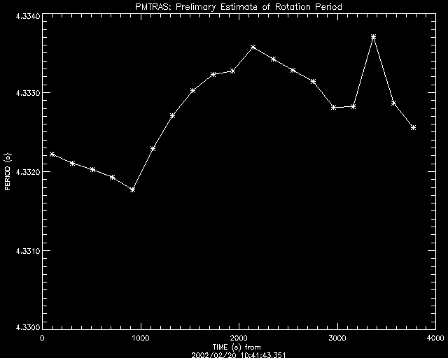
from the displayed curve, you can get the spin period. For 2002 02 20 11:06:30:20 it is 4.3329 seconds.
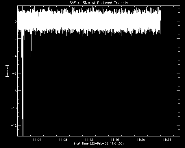
intervals without SAS solutions are printed out. the plot shows the size of the triangle of the SAS solution, should be around zero. for this time interval, there are no gaps, but some bad SAS solutions in the beginning (~11:02). after 11:04 everything is fine. at the moment, better do not use SAS solution close to hessi eclipse (+-10 minutes).
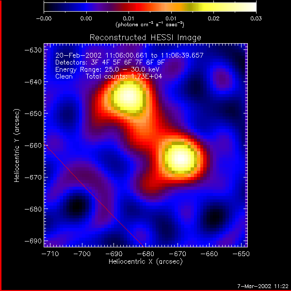
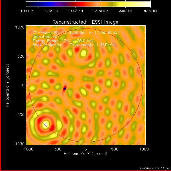
first we make a low resolution (grid 8) image (backprojection) of the full Sun to find the position of the flare. REMARK: absolute flare positions are not available at the moment (march 5, 2002), but the radial position of the flare is ok.
time_range (gives time range relative to obs_time_interval) is selected to
be multiples of the spin period: time_range=[14.*ttt,23.*ttt] is the time interval
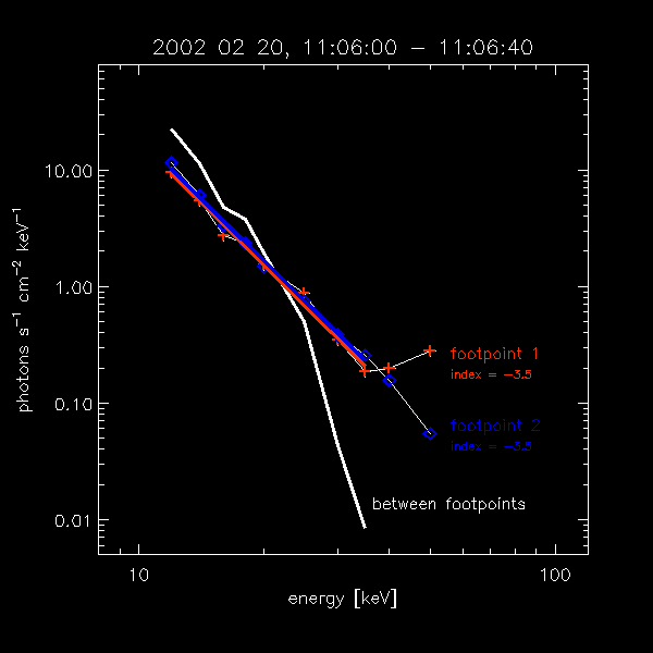
of the HXR peak, check light curves
IDL> o=hsi_image()
IDL> o-> set, as_spin_period = ttt
IDL> im=o->getdata( image_alg='bproj',obs_time_interval=tr,
pixel_size=[16.,16.],image_dim=[128,128],xyoffset=[0,0],
det_index_mask=[0,0,0,0,0,0,0,1,0],
energy_band=[12.,25.],time_range=[14.*ttt,23.*ttt])
IDL> o->plotman
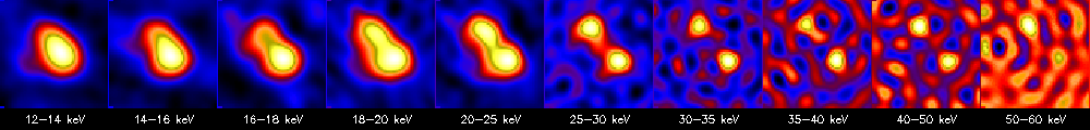
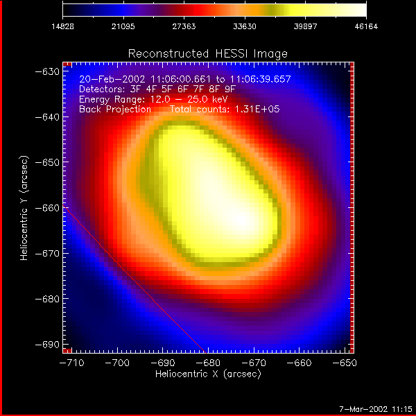
now we know the position and we can make higher resolution images around the flare source. grid 3-9 are calibrated so far.
Ed Schmahl pointed out: " ... once in a while the mirror source can be brighter than the real source. Then you have to zero in and make maps with finer collimators with different collimator phases. With collimators 4 and 5 the mirror source will appear dark. This is going to make automatic flare finding more difficult that we had hoped. The problem arises because (a) the pointing is too stable (!) and (b) Alex aligned the coarse subcollimators too well (!)."
"Another "gotcha" is getting a constant vector for the roll_angle if you use a start value too close to the beginning of an orbit. Maps will appear as a single modulation pattern. Apparently, whatever program fills in fake roll_angles in the absence of true RAS data gets confused and gives you roll_angles that are all one value. The fix, of course, is to start a minute or two later."<\p>
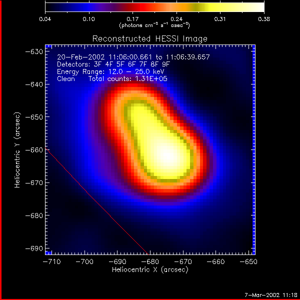
and we can clean it:
IDL> cl=o->getdata(image_alg='clean',/clean_mark_box,clean_niter=200)
IDL> o->plotman
and now we can play around and have fun:
IDL> cl25=o->getdata(energy_band=[25,30])
IDL> o->plotman