Flare Footpoint Aymmmetries
Schmahl, Pernak & Hurford
The hard X-ray domain is not usually where one would think of finding
diagnostics of coronal magnetic fields, but the shape and cross sections of
the flare loops that constrain high energy electrons contain useful
information about magnetic fields not obtainable in any other way. One
example of such information comes from HXR observations of the footpoints of
flare loops, visible as elliptical features in flare images at energies
where thick-target emission dominates. It has been known for over a decade,
largely from HXT, but also radio, that footpoint fluxes are seldom equal, and
that asymmetry is the rule rather than the exception. It is possible that
the asymmetry is just due to an asymmetric injection of high energy electrons,
but there are new RHESSI observations that seem to favor a symmetric injection..
Back in 1979, before hard X-ray imaging became a reality, Melrose and
White offered up a trap/precipitation model that suggested that the
flux asymmetry of hard X-ray footpoints in flaring loops would be
caused by a magnetic asymmetry. In this model, magnetic convergence
at the footpoints should mirror a fraction of streaming and spiraling
electrons (green spirals in the figure below), and for electrons with
small pitch angles (i.e moving more parallel to the magnetic field),
where the mirror point lies in the chromosphere, hard X-ray emission
would be emitted from regions whose area was that of the trapping
magnetic flux tube.
Figure 1 Cartoon of trap/precipitation model for symmetric & asymmetric loops.
The footpoint (red) with stronger magnetic field mirrors a larger fraction of
the electrons than the other footpoint, and so fewer thick-target hard X-rays
are emitted from that footpoint. Thus hard X-ray footpoint flux should
correlate negatively with magnetic field strength. As a function of position
along the loop, the cross sectional area of the magnetic loop will be
inversely proportional to the magnetic field strength, so the footpoint area
ratio should equal the reciprocal of the magnetic footpoint field ratio, and
hard X-ray flux should correlate positively with footpoint area.
The trap/precipitation scenario led many HXT workers to compare hard-X-ray
footpoint flux ratios with magnetic fields determined from magnetograms. Taro
Sakao wrote part of PhD thesis on this subject in 1994 at the University of
Tokyo, and found that out of 5 flares that he studied, the footpoint with
higher magnetic flux (B) was weaker in hard X-rays. This was a vindication of
the trap/precipitation model. Later HXT studies by Goff et al. came to a
different conclusion than Sakao. Out of 32 flares, only 14 showed the low-B,
bright X-ray association. But these studies suffer from the fact that the
magnetic fields were measured at the photospheric level, rather that at the
chromospheric level where the hard X-rays were emitted. Also, with two
different instruments, one has different cadences, resolutions, and pointing
systems. So if hard X-ray imaging could determine the area of the footpoints,
the asymmetry in both flux and area (inverse magnetic field) could be seen
without ambiguity. Unfortunately this was not possible with HXT, nor, until
recently, with RHESSI.
A new method of imaging
In 2006 it became possible to make quantitative area measurements
with RHESSI data. The method makes use of "visibilities", which are
the calibrated amplitudes and phases of the modulation profiles. (A
discussion of RHESSI visibilities should be a subject of a future RHESSI
Nugget.) To apply visibilities to imaging, one makes an image model
with adjustable free parameters. A Fourier transform then provides
model visibilities which can be compared with the observed visibilities.
The free parameters are adjusted until a good (or the best
possible) fit is obtained. This "visibility forward fit" technique is
very fast--faster than Clean--and provides error bars derived from the
count statistics and the estimated hardware uncertainties, all fed through the
nonlinear fitting process. Some examples of maps are shown
below.
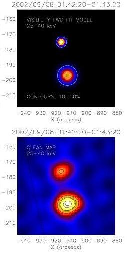
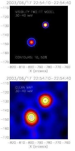
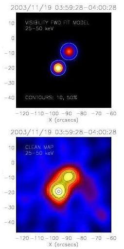
Figure 2. Three examples of Visibility Fwd-fit (top row) and Clean
for the same times and energies. Note the agreement of the two methods
for the positions of the footpoints, but the frequent difference in
the Visibility Fwd-fit and Clean sizes.
Example of fit to an amplitude profile
Here we show the amplitude profile of a double-component RHESSI flare as a
function of both subcollimator (SC) and position angle (PA). The horizontal
axis is SC+PA/180, so for example, for abscissa values between 6 and 7, the
data are for SC 6 with PA between 0 and 180 degrees.
The bumps and wiggles are caused by the sources "beating" against each
other as the collimator slats rotate from positions where both sources are
visible to positions where only one is visible. The curve was fit by a model
with 8 parameters describing two circular Gaussians. The χ2
was found to be about 1, where the sigmas are derived from count statistics
and a 2% instrumental uncertainty.
Figure 3. Observed (x), fitted
(-) and residual (squares) amplitudes for one double footpoint flare.
There are a number of ways to test the fit of such models to the
data, and its uniqueness:
- General agreement of the model with the
observed bumps/wiggles in both amplitude and phase;
- location and depth of
minima in cross sections through the multi-dimensional χ2
space;
- residual maximum as as a fraction of the maximum in a visibility
back-projection;
- the sensitivity of the result to increasing the number
of free parameters;
- the similarity of the fwd-fit map to images obtained
by other means.
Some observed widths and fluxes
A sample of 26 double-component events FWHM plotted against flux shows
that the brighter component is also broader, as predicted by Melrose &
White, in the large majority of cases (23 out of 26). Relatively
small error bars give us confidence in the result.
Figure 4. Flux and FWHM of components in double-footpoint flares
Each colored bar represents a separate flare or flare interval, with
squares at the bar's end showing the flux and fwhm of that component. Crosses
at the end of each bar show estimated 1-sigma errors in flux or fwhm for
each component. Note that the slope is positive for all but 3 bars; only one
(white bar) of those is significant at the 2 or 3 sigma level.
Our conclusions
We have found that the brighter footpoints are broader than the
fainter conjugate footpoint in 23 of the 26 flare intervals studied.
This is shown by the predominantly positive slopes of the line
segments joining the footpoint parameters (flux, fwhm) in the above
figure. This result validates the Melrose and White prediction, and it
is in general agreement with Sakao's result, although the width-flux
correlation is better (23/26) than his magnetic field-flux correlation
(4/5), and significantly better than Goff et al's result (14/32). The
possibility of an asymmetric injection as an explanation for flux
asymmetry now seems to be unlikely on the basis of this strong
correlation of footpoint flux and area, since if the injection were
highly asymmetric in a random way, the correlation would be close to zero.
Systematics in the determination of areas must be carefully
considered, although no one so far who has seen these results (at 3 meetings)
has suggested any instrumental mechanism that might make
brighter sources look broader to RHESSI.
Comparisons with magnetograms can check the sign of the width
asymmetry. But there are often large horizontal (and perhaps
vertical) gradients in photospheric magnetic fields that might make the
correspondence with footpoint area less clear.
Microwave observations can help estimate the degree of trapping
to check the consistency of our results, although the microwave maps
necessarily have different (usually lower) resolution, and are generated by
higher energy electrons, which leads to other complications.
It is also possible to draw conclusions from these width-flux
asymmetries regarding the pitch angle distributions and the loss-cone
angles, but that's another story to be told later.