Visibilities à la Fourier

RHESSI is a Fourier imager, which means that it obtains amplitudes and phases (a.k.a. "visibilities") of the X-rays that it modulates. This particular design was driven by many forces, not the least of which was the mantra "faster, better, cheaper" which put strong cost and size constraints on the small explorer (SMEX) satellites of the 1990s. Previous solar instruments that used Fourier techniques were Hinotori, HEIDI, and HXT, but RHESSI has unique new Fourier/visibility-based capabilities that are only now beginning to be exploited.

What does Fourier have to do with imaging? The 18th century mathematician Jean Baptiste Fourier discovered the principle that any signal can be broken up into a superposition of sines and cosines, or the equivalent amplitudes and phases, but he did not himself invent Fourier imaging. Applications of Fourier methods to imaging had to wait until the late 19th century when the amplitude and phase pairs of optical interferometry came into use, and these pairs came to be known as visibilities, as in "fringe visibility". Later in the 20th century radio interferometry used the same entities, and now hard X-ray astronomers have joined the visibility game.

How do we create visibilities?

To get hard X-ray sines and cosines is difficult, but RHESSI uses a good approximation, triangular waveforms. In the ideal case--constant background, thin grids, and high photon rates-- the modulated waveform generated by photons incident on one of RHESSI's sub-collimators has a triangular profile (Fig. 1). The amplitude of the waveform is proportional to the intensity of the beam and its phase and frequency depend on the direction of incidence. For complex sources, and over small rotation angles, the amplitude and phase of the waveform provide a direct measurement of a single Fourier component of the angular distribution of the source. Different Fourier components are measured at different rotation angles and with grids of different pitches.

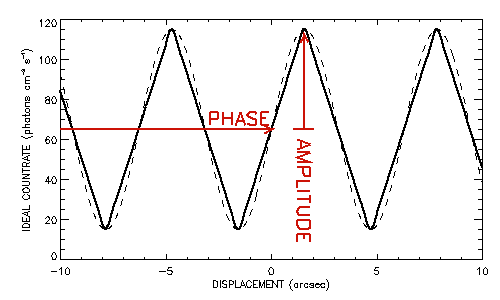Fig. 1 Ideal hard X-ray grid response (solid curve), with its associated fundamental sinusoid (dashed curve).

From time tags to visibilities

We illustrate the end-to-end process of computing visibilities for a particular flare interval, a single subcollimator, and a single energy band. The primary RHESSI data are photon time tags and pulse heights, which must be transformed in various ways before imaging is possible. RHESSI's time tags and pulse heights for a selected 100-ms interval are shown in Fig. 2a. These time tags have not yet been binned in energy or time, so they are difficult to interpret by eye, but several cosmic-ray-produced gaps are evident.

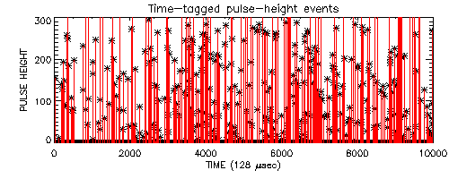Fig 2a Time-tagged pulse heights

A sequence of basic (linear) operations must be performed on these data to convert them to visibilities. The next step is to bin the data in energy and in uniform roll-angle bins, as shown in Fig 2b.

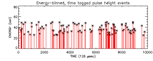
Fig 2b Energy-binned pulse heights.

The next step is to "histogram" the time tags into time bins, as shown in Fig 2c for 3 rotations.

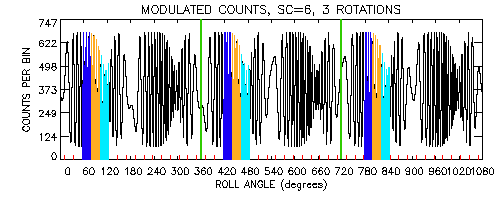
Fig 2c RHESSI modulation profile. The green vertical lines mark the boundaries of spacecraft rotations, and the red tick marks indicate the roll bins selected for phase-bin stacking. Three sets of rollbins are identified by the colors blue, orange, and cyan.

We now progress further towards constructing visibilities by binning the modulation cycles into roll bins, which are then binned again into 12 aspect phase bins. In this case there are 16 roll bins, three of which are outlined in color (blue, orange, and cyan) in each rotation. After phase binning, each of these rollbins can be co-added.

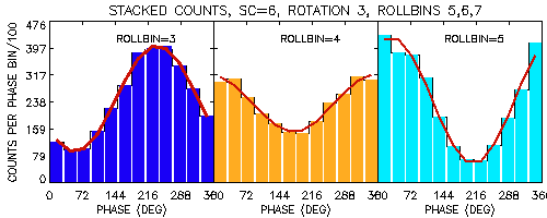
Fig 2d Stacked roll bins #3,4 & 5 taken from the three selected regions shown in corresponding colors in the previous figure.

This process, called "stacking" increases the S/N ratio and provides a platform for computing amplitude and phase.. This generally improves the aspect phase coverage because the angular drift of the telescope causes the aspect phase to differ from one rotation to the next. After stacking we fit sinusoids to the profiles (red curves in Fig 2d).

In order to calibrate the parameters generated by the fits, a number of corrections must be made. The grids have a finite thickness, which produces internal shadowing and modifies the triangular-like response; this also causes a decline of transmission as a function of the off-axis distance; the grid slats are not all perfectly aligned parallel to the optical axis, which leads to a "venetian blinding" effect, which makes even and odd half-rotations unequal; and there are detector-to-detector sensitivity differences. Fortunately, RHESSI was calibrated in many ways before launch, and the instrument has many self-calibration capabilities, so all of these effects can be calibrated out. Using the RHESSI calibrations, one may remove the instrumental dependence and convert the sinusoids to photon rates.

The final steps in constructing visibilities are to output the amplitudes and phases of the fitted sinusoids, and compute error estimates based on photon statistics and instrumental systematics. Fig. 2e shows the computed amplitudes in the upper panel, and the visibility phases in the lower panel.

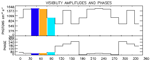
Fig 2e Visibility amplitudes and phases derived from the stacked counts in Fig, 2d. Roll bins #3,4 & 5 taken from the three selected regions are shown in the same colors as the previous figure.

Note that the visibility amplitudes are in units of photon flux, unlike the stacked modulation profiles, which are in counts per bin. Since the calibrations have been applied, the visibilities are very nearly independent of the instrument. The importance of this instrumental independence is hard to overestimate. It makes it possible, for example, to use radio imaging techniques such as MEM for RHESSI imaging, and to do forward fitting (see earlier nugget). We list several other applications of visibilities later.

RHESSI visibility amplitudes

Above, we showed data for only a single subcollimator. But RHESSI's great imaging power results from its coverage of a wide range of spatial scales with its 9 subcollimators. Here (Fig. 3) we show the amplitude dependence as a function of both subcollimator (SC) and roll angle (PA). The x axis is a linear combination of both variable in the form SC+PA/180. Thus, for example, the roll angles 0 to 180 degrees are shown for subcollimator 6 for x between 6.0 and 7.0.

The observed amplitudes are indicated by blue crosses and their associated estimated standard errors are shown by vertical error bars. Note the variable amplitude as a function of roll angle for each subcollimator. This variation is caused by the "beating" of the two flare sources against each other. Note also the gradual falloff of amplitude as the subcollimators become finer (towards smaller x). This falloff is the result of the finite size of the sources. When the angular pitch is smaller than the source size, the modulation amplitude is reduced (and error bars become larger).

The solid red curve shows the visibility computed for a model given by two Gaussian sources. For subcollimators 2-9, the model fits the observations quite well. For the finest subcollimator, the angular pitch is much smaller than the source size, and the amplitudes are essentially indeterminate. The residuals, shown by squares, are relatively small for all subcollimators above 1.

Amplitude profiles such as this (and of course, phase profiles, which, for reasons of nugget space we do not show) are invaluable for diagnosing source structure of many kinds.

Fig. 3. Observed visibility amplitudes (blue crosses) for a flare interval as a function of subcollimator (SC=1-9) and position angle (PA=0-180°) of the grids. Each of the 9 vertical panels shows the amplitude as a function of PA for one subcollimator (labeled by red digits below the X axis). The red curve represents a model using two Gaussian sources, and the green squares show the residuals relative to the model. For a given subcollimator (6 and 7 are good examples), the amplitude rises and falls sinusoidally while the grids rotate from PA=0 to PA=180°. In general, such sinusoidal variation indicates an extended or double source.

What use are RHESSI Visibilities?

Aside from the advantages that RHESSI visibilities are a highly compact, device-independent representation of the data, there are several other advantages to creating them. For one, making maps can be greatly sped up by using highly optimized radio astronomy programs. For another, one may reliably determine source sizes using a visibility forward-fit routine. Other barely exploited advantages are

• Mapping in the 7 keV Fe line;
• Mapping in the sum of nuclear lines;
• Mapping in terms of photon energy, not detected energy;
• Mapping separately in nuclear lines and the continuum;
• Improved pileup corrections for hard X-ray images
• Enhancing statistical sensitivity by weighting
• Improving iterative processing

Another important, already-exploited use is self-calibration of phases. By means of such self-calibration it will become possible to utilize the 2nd and 3rd harmonics of the near-triangular RHESSI waveform (Fig. 1). Up until now, we have used only the fundamental sinusoids, but the higher harmonics will provide more complete coverage of the Fourier plane for better imaging and higher resolution, as good as ~ 1 arcsec.

Acknowledgments

The RHESSI software team, particularly Richard Schwartz and Rick Pernak, have helped bring us into a renaissance of visibilities. without their continuing assistance, the team would still be in the dark ages of Fourier imaging.