Polar Representations

Another strategy is to go into polar coordinates. We show that this gives savings in both time and storage. (It is important to note that the method does not assume that the spin axis remains fixed!) We must convert the Fourier transform from rectangular coordinates (x,y) to polar coordinates $(r,\theta)$ in map space, and (u,v) to $(q,\phi)$ in visibility space. The rectangular form is:

$$g(x,y)= \int_{-\infty}^{\infty}\int_{-\infty}^{\infty} f(u,v)\ e^{2\pi i (ux+vy)} du dv \eqno{(2)}$$

The conversion from rectangular to polar coordinates can include offsets from a nominal center:

$$x=r\ cos(\theta) + a(\phi)$$

$$y=r\ sin(\theta) + b(\phi)$$

where a and b can be arbitrary functions of $\phi$ (derivable from the HESSI aspect solution). Using this, equation (2) becomes:

$$g(r,\theta) = \int_{0}^{\infty} q\ dq \int_{0}^{2\pi} d\phi\... ...lpha(\phi)} \ e^{2\pi i r q \ cos(\theta - \phi)} \eqno{(3)}$$

and the phase factor $\alpha$ represents the phase offset from the nominal rotation axis:

$$\alpha = 2\pi (a\ cos(\phi) + b\ sin(\phi)).$$

As a function of radius q, $f(q,\phi)$ is a sum of Dirac delta functions, so the radial integrals are trivial, and we are left with 9 azimuthal integrals:

$$g(r,\theta) = \sum_{j=1}^9 q_j \int_{0}^{2\pi} d\phi\ f_j(\p... ...ha(\phi)} \ e^{2\pi i r q_j \ cos(\theta - \phi)} \eqno{(4)}$$

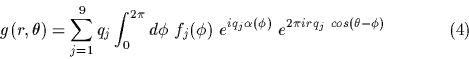
The visibilities' azimuthal dependence can be represented as a Fourier series with the number (N_j) of (complex) coefficients given by column 2 or 3 in Table 1. N_j is large when j=1 and is 81 times smaller when j=9:

$$f_j(\phi) e^{i q_j \alpha(\phi)} = \sum_{k=-{N_j}}^{N_j} f_{jk}\ e^{i k\phi} \eqno{(5)},$$

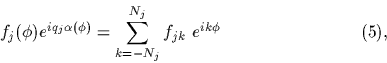
where N_j is the number of visibilities for the j th subcollimator.

Plugging (5) into the Fourier integral (4) above gives:

$$g(r,\theta) = \sum_{j=1}^9 q_j \sum_{k=-N_j}^{N_j} f_{jk} ... ...\ e^{2\pi i r q_j \ cos(\theta - \phi) +i k \phi} \eqno{(6)}$$

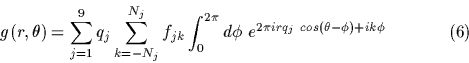
Then using the integral representation of the Bessel function J_k, we are left with:

$$g(r,\theta) = {{1} \over {2\pi}} \sum_{j=1}^9 q_j \sum_{k=-N... ...j} f_{jk}\ J_k(2\pi r q_j)\ e^{i k (\theta+\pi/2)} \eqno{(7)}$$

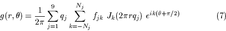
Here we have 9 Fourier transforms of the $f_{jk} J_k(2\pi r)$ arrays. These arrays are not square, and will be of size $2N_j \times M$,where N_j is the number of points on the j th UV circle and M is the map size. These arrays are somewhat smaller than in the direct representation (Sect. 3), but they scale the same way. For the case M=360, the arrays will be about 4 times smaller, and are smaller by even larger factors than the arrays in the rectangular representation.

Furthermore, all the Fourier transforms can be done using FFTs, because $\phi$ is distributed uniformly around the UV circles. (In the direct representation the u_k and v_k are not evenly spaced in azimuth, making FFTs impossible.) So the polar approach has potential advantages for both speed and storage.

It is worth looking for a way to speed up the Bessel function calculations, since they are the limiting factor here. In fact, a factor of 2 speedup can be gotten by computing only the even order Bessel functions, and using the recurrence formula for the odd orders:

$$J_{\nu-1}(z) = (z/2\nu) (J_{\nu-1}+J_{\nu+1})$$

Extensions of this trick lead to about 2 orders of magnitude speedup of the Bessel function calculations. IDL tests show that it is possible to use this ``downward'' recurrence relation to produce an array of Bessel functions about 50 times faster than the stock IDL routine. Effectively each of the Bessel coefficients in equation (7) can be produced in a few floating-point operations, instead of the estimated 450 for repeated calls to IDL's beselj(x,n). In practice, one calls beselj(x,n) only twice, and creates each of the remaining Bessel functions by one multiplation, one division, and one addition. Tests show that this is a very stable recurrence.

One minor disadvantage of using polar coordinates is that in projected solar coordinates the maps will be bounded by non parallel lines and circular arcs, but this can be mitigated by interpolating them onto square arrays after the image processing is complete.

An example of an array of Bessel Functions