|
Other RHESSI |
|
|
|
|
|
|
|
|
|
|
|
|
HESSI Tutorial on Forward-Fitting : I. Standard Example
This tutorial is intended for HESSI users who want to use the forward-fitting method in the IDL SSW environment to reconstruct HESSI images. For basic information on image processing see tutorial written by Chris Johns-Krull (http://hessi.ssl.berkeley.edu/~cmj/hessi/doc.html). We start with the standard example of simulated data that is generated in the HESSI software. We explain various steps how the forward-fitting tool can be used to reconstruct and improve an image. The resulting numbers serve as a rough guide, but may vary in different runs, because the data simulator contains a random generator and Poisson noise.
We initiate an object reference, we choose the image algorithm,
reconstruct the image, and plot the resulting image:
o = hsi_image()
o -> set,image_algorithm='forwardfit'
im = o -> getdata()
o -> plot
Every setting of control parameters can also be specified by keywords, e.g.
im = o -> getdata(image_algorithm='forwardfit',/plot).
The resulting image shows a gaussian source at location [600,200] arcsecs offset from
the Sun, reconstructed with detectors 4-8 and in the energy range 12-25 keV.
Let us check the image control parameters, which we extract into the structure p,
and check parameters that are relevant for optimization of our image processing:
p = o -> get()
print,p.det_index_mask
.... e.g. [0,0,0,1,1,1,1,1,0,...]
print,p.energy_band
.... e.g. [12,25] keV
print,p.time_range
.... e.g. [0,4] s
print,p.xyoffset
.... e.g. [600",200"]
print,p.image_dim
.... e.g. [64,64]
print,p.rmap_dim
.... e.g. [65,67]
print,p.pixel_size
.... e.g. [4",4"]
print,p.sim_pixel_size
.... e.g. 1"
print,p.sim_xyoffset
.... e.g. [600",200"]
print,p.sim_model_ptr(0)
.... e.g. [1.0,0.5",1.0",-11.5",-11.5",0 deg]
print,p.sim_model_ptr(1)
.... e.g. [1.0,0.5",1.0",0.5",0.5",0 deg]
print,p.sim_photons_per_coll
.... e.g. [1000,...;0,...;0,...]
print,p.n_gaussians
.... e.g. 1 (number of gaussian components)
print,p.n_par
.... e.g. 4 (number of free parameters per component)
The simulation model parameter SIM_MODEL_PTR
is a structure that contains the amplitude, the x and y gaussian
widths, the x and y position, and the tilt angle. In our standard example we see that the
image contains two gaussian sources with equal amplitude (1.0), elliptical shapes (x-width=0.5,
y-width=1.0), one source at position [x,y]=[-11.5",-11.5"], and the second source at position
[x,y]=[+0.5",+0.5"], relative to the xyoffset=[600",200"]. The photon counts per collimator
is 1000 cts/s for the 9 front detectors, and 0 cts/s for the rear detectors.
There are a number of output parameters provided after an image reconstruction
with the forward-fitting algorithm has been completed. You can access them by:
print,p.chi_ff
.... C-statistic of 9 detectors, e.g. [0,0,0,1.14,1.11,1.18,1.08,1.35,0]
print,p.chiav_ff
.... average of C-statistics from non-zero detectors, e.g. C=1.17
print,p.phot_sec
.... incident photon rate, e.g. R=597 photons/sec
print,p.peak_flux
.... gaussian amplitude, e.g. A=3.20 photons/sec/cm^2
print,p.coeff_ff
.... coefficients of forward-fit, e.g. [1.00, 6.30", -6.02", -5.20"]
The solution is parameterized with 4 coefficients of a single gaussian component: the normalized amplitude coeff(0,0)=1.00 (which corresponds to a flux of A=3.20 photons/sec/cm^2), the gaussian width of coeff(1,0)=6.30", and the coordinates of the centroid at [x,y]=coeff(2:3,0)=[-6.02",-5.20"]. We see that the single-gaussian fit located an intermediate position between the two true source locations, with a gaussian width that is comparable with the distribution of the two combined sources.
Given the information about the simulated image we know that 2 gaussian components
should be used for the forward-fitting model. In real data, where the true source
structure is not known, we would use either the chi-square information from a
preliminary forward-fitting run or another quick imaging method (e.g. back-projection) to
guess a suitable number of source components. A perfect model would yield a chi-square
in the range of chi2=0.95...1.05. If the resulting chi2 is higher, it is justified to
increase the number of gaussian components. In the run above we find, e.g. a value of
C=1.17, which suggests to increase the number of free parameters, either a higher number
of source components (n_gaussians > 1) or a higher number of parameters (n_par > 4).
As a first attempt, we change the default value for the number or sources from N_GAUSSIANS=1
to N_GAUSSIANS=2. In addition, from the first run we see that we see that the source is very compact,
so we can reduce the field-of-view from 64x4"=256" to, say 64x1"=64". It is also advisable
to use the finer detectors for small sources that could be otherwise unresolved in a
compact source, so we enable all detectors a priori (the forward-fitting will
automatically select a subset of detectors with significant counts from the preset detector
set DET_INDEX_MASK). The photon statistics can also be improved by considering a larger
energy range, say E=[6,300] keV instead of the default range E=[25,50] keV.
An improved run may be attempted with:
o = hsi_image()
o -> set,image_algorithm='forwardfit'
o -> set,n_gaussians=2
o -> set,pixel_size=[1,1]
o -> set,image_dim=[64,64]
o -> set,energy_band=[6.,300.]
o -> set,time_range=[0,4]
o -> set,det_index_mask=bytarr(9)+1B
im = o -> getdata()
o -> plot
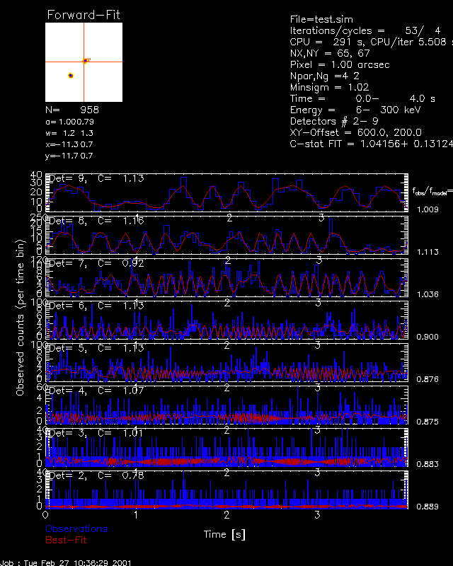
For this test we find the following values (you will get slightly different values because
there is a random generator used for the simulation of incident photons):
p = o -> get()
print,p.n_gaussians
.... e.g. 2 (number of gaussian components)
print,p.n_par
.... e.g. 4 (number of free parameters per component)
print,p.chi_ff
.... C-statistic of 9 detectors, e.g. [0.00,0.78,1.01,1.07,1.12,1.13,0.91,1.15,1.12]
print,p.chiav_ff
.... average of C-statistics from non-zero detectors, e.g. C=1.04
print,p.phot_sec
.... incident photon rate, e.g. R=959 photons/sec
print,p.peak_flux
.... gaussian amplitude, e.g. A=4.77 photons/sec/cm^2
print,p.coeff_ff(*,0)
.... coefficients of first source, e.g. [1.00, 1.19", -11.34", -11.69"]
print,p.coeff_ff(*,1)
.... coefficients of second source, e.g. [0.99, 1.34", 0.69", 0.73"]
The coefficients contain the following information: [amplitude, width, x-position, y-position].
So, we found the first Gaussian component with amplitude=1.0, width=1.19",
x,y=[-11.34",-11.69"], and the second gaussian component with amplitude=0.99, width=1.34,
x,y=[-0.69",-0.73]. Comparing these solutions with the simulation parameters we find agreement
of the location within ~0.2", which is satisfactory given the pixel resolution of 1".
Further insights into the fidelity of image reconstruction can be obtained by reconstructing the same image with other algorithms. Some test image comparisons are shown for backprojection, clean, and forward-fitting on the web-page:

