|
Other RHESSI |
|
|
|
|
|
|
|
|
|
|
|
|
HESSI Tutorial on Forward-Fitting : IV. Simulation and Forward-fitting of Loops
In this tutorial we demonstrate the simulation and image reconstruction of images with loop-like features. Source structures with geometries of spherical gaussians and elliptical gaussians can be simulted with the so-called (predefined) "gaussian source structure":model = {gaussian_source_str}
For simulation of loops we generalized this structure by including an additional parameter, the curvature parameter c, which is defined by the inverse curvature radius r, normalized by the gaussian width w_x, to make it dimensionless: i.e. c=w_x/r. This definition has the value c=0 for straight elliptical gaussians, typical values of c~0.01...0.1 for weakly curved loops, and c~0.1...1 for strongly curved loops. This additional curvature parameter is included in the structure {curved_gaussian_source_str} (implemented in SSW by Jim McTiernan on March 9, 2001). Here an example of a model definition that defines a map with a single loop with a curvature radius of r=25" and gaussian width w_x=5.0", i.e. curvature parameter c=w_x/r=5"/25"=0.2:
model = {curved_gaussian_source_str}
model.amplitude = 1.0
model.xysigma = [5.0, 1.0]
model.xypos = [-25.0, -25.0]
model.tilt_angle_deg = 60.0
model.curvature = 0.20
Then define an object, set the simulation model, and reconstruct the image with forward-fitting (use N_PAR=7 to indicate that you want geometries with curved ellipses):
o = hsi_image()
o -> set, sim_model = model
o -> set, sim_pixel_size = 2.0
o -> set, sim_photons = 10000
o -> set, det_index_mask = byte([0,1,1,1,1,1,1,1,1])
o -> set, image_alg = 'forward'
o -> set, n_par = 7
o -> set, nitmax = 30
image = o -> getdata(/plot)
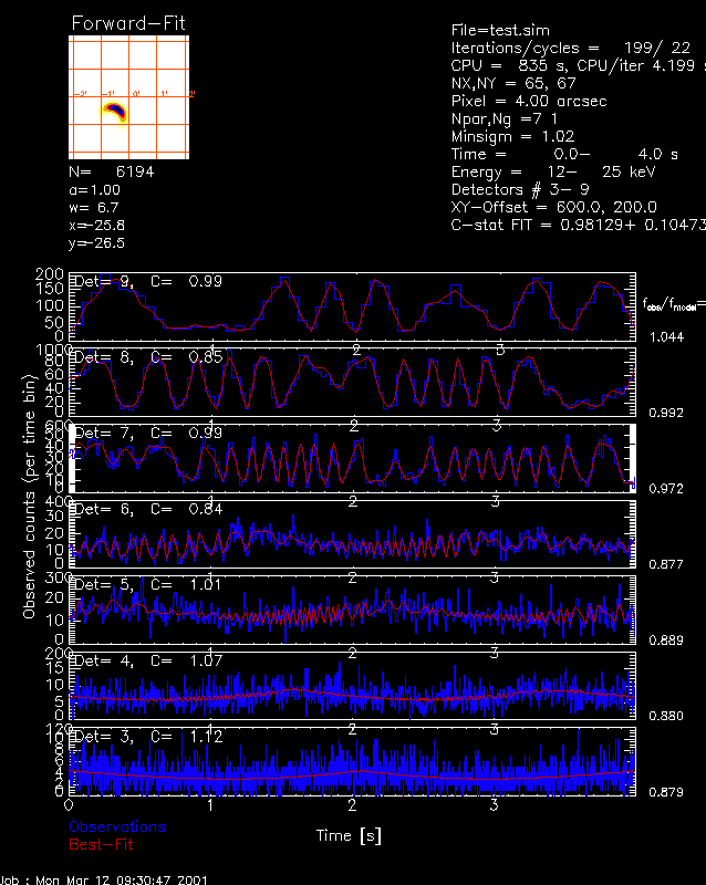
The result might look like this:

You might be interested to verify how good the forward-fitting retrieved the
model parameters:
p = o -> get()
print,p.coeff_ff
.... coefficients of forward-fit, e.g. [1.00, 6.69", -25.79", -26.49",2.01,59.20,0.26]
The definitions of the 7 coefficients are:
print,p.coeff_ff(0)
.... amplitude a= 1.00
print,p.coeff_ff(1)
.... gaussian width w_x=6.69" "
print,p.coeff_ff(2)
.... x-position x=-25.79""
print,p.coeff_ff(3)
.... y-position y=-26.49""
print,p.coeff_ff(4)
.... eccentricity e=w_x/w_y-1=2.01 -> gaussian width w_y=w_x/(1+e) "
print,p.coeff_ff(5)
.... tilt angle in degree t=59.20
print,p.coeff_ff(6)
.... curvature parameter c=w_x/r=0.26 -> curvature radius r=w_x/c=
The comparison with the model parameter yields:
print,model.amplitude, p.coeff_ff(0)
.... 1.0, 1.0
print,model.xysigma(0),p.coeff_ff(1)
.... 5.0", 6.7"
print,model.xysigma(1),p.coeff_ff(1)/(1+p.coeff_ff(4))
.... 1.0", 2.2"
print,model.xypos(0),p.coeff_ff(2)
.... -25.0",-25.8"
print,model.xypos(1),p.coeff_ff(3)
.... -25.0",-26.5"
print,model.tilt_angle_deg,p.coeff_ff(5)
.... 60.0 deg, 59.2 deg
print,model.curvature,p.coeff_ff(6)
.... 0.20, 0.27

