How does the decimation correction work?
How do I avoid memory allocation errors when accumulating long time intervals for spectra?
Can I estimate how much memory I need?
I run out of memory when writing the full response matrix with binning code 16.
I run out of memory when creating images.
Can I combine front and rear detectors for spectra?
How can I subtract background from a different orbit from the flare?
Can I merge spectrum FITS files that were created separately?
How do I subtract background in a different attenuator state from the flare intervals?
Can I remove the jumps caused by attenuator and decimation state changes in a lightcurve?
How can I recover the true incident flux modulation?
How can I write a SPEX FITS file with energy bins defined on channel boundaries?
How can I get channel edges in keV?
Are attenuator and decimation changes corrected for in images?
Is pileup corrected for in images?
How do I read a RHESSI image FITS file?
How do I read a RHESSI image cube FITS file?
Can I write a RHESSI image cube FITS file without using the GUI?
Can I combine several image cubes into one image cube FITS file?
I want to extract an image from the GUI to work with outside of the GUI.
How can I compute the flux in a region for all images in an image cube FITS file?
How can I use the "Image Flux" output file?
How can I plot the time evolution of the flux of a source region?
How do I get the energies and times for a spectrum or lightcurve?
How do I get the x and y axes for an image?
If I know recent software changes aren't working, how can I remove the atest directory?
How do I determine which subcollimators to use when making a map?
Should I use subcollimator 9 when making a 128" x 128" or smaller map?
How do I get the Point Spread Function for a given collimator?
How can I send multiple plots to the same plotman widget?
How can I get or plot the aspect solution?
How can I find the spin axis and spin period?
How do I work
with the hessi spacecraft time format?
Front decimation correction is turned on by setting the decimation_correct parameter to 1.
Rear decimation correction is turned on by setting the rear_decimation_correct parameter to 1.
o -> set, /decimation_correct, /rear_decimation_correct
To see whether decimation correction was needed, look at the decim_table info parameter.
These are the factors used in determining front decimation correction:
The decim_state flag only indicates the amount of decimation. So for decim_state 2, 1/2 counts below the threshold channel are eliminated at random. For state 4, 3/4 counts are removed, etc.
The threshold channel is the same for all front segments. This is determined by the decim_state and the decim_channel set in an onboard table and depends on the current atten_state and ssr level (ssr_state). As the atten_state increases, the decim_channel also increases to keep the decimation effective in reducing the flow of counts into the memory. As the memory becomes more filled, ssr_state increases and the decimation needed increases. The table versions are found in the version_idpu flag in the packet header and obs_summ flags. The spectrogram methods for decimation take the idpu_version, ssr_state, and atten_state as inputs for hsi_front_decimation to determine the decim_weight and decim_channel.
With the decim_channel in hand, the decim_energy can be found using the gain tables maintained by David Smith and Peter Schroeder.
The decimation correction is applied to the livetime as it is effectively identical to deadtime in its action and this method preserves the integrity of the count statistics. So for N counts, the standard deviation is sqrt(N). For energy bins lying below the decim_energy the decimation correction is straighforward - the livetime is divided by the weighting factor of decim_state N, i.e. N.
There is one energy bin that is the boundary between applying 1/n to the livetime and leaving it undisturbed. At this bin the decim_energy will fall somewhere within an energy_channel and the method computes a spectrally weighted average that it uses in computing the weighting factor. The spectrum used for the weighting is a count rate spectrum based on a nominal flare spectrum multiplied by the diagonal detector response. The attenuator state is included in this computation.
So the determinants of the correction are the weighting and energy channels for each front segment and the correction is only valid for time intervals where none of the inputs to hsi_front_decimation has changed, specifically the idpu_version, the atten_state and the ssr_state. Since idpu_version changes on the order of months to years, only changes to atten_state and ssr_state are important during flares.
To look at the structure that determined the decimation correction using all of the above considerations look at the function decim_time_range() which is a method of both hsi_spectrum and hsi_binned_eventlist. This method should only be called after processing a data selection and it returns a structure with the times, weights, energies, and correction factors that can easily be inspected.
Rear Decimation correction operates off of values found in the observing summary. It runs off of tables that predict times of high particle fluxes and is not directly keyed to the ssr_level. The flags used are obtained from the changes() method and have the fields rear_dec_chan_128 and rear_dec_weight. The weight is usually 4 or 6 and the channel value must be multiplied by 128 to find the threshold for decimation. The times and corrections can also be found using the decim_time_range() method of hsi_spectrum or hsi_binned_eventlist with the rear_decim_correct keyword set.
When accumulating long time intervals with many time and/or energy bins in the spectrum object, you may run out of memory. In order to get around this, you can make several separate accumulations, write a FITS file for each and then merge the FITS files together using the FITS paster routine.
To get a rough estimate of how much memory is required to accumulate an image or spectrum with the parameter options you have set into an object, use the hsi_est_memmax function as follows:
print, hsi_est_memmax(object)
The result is the number of bytes needed. The object argument is one of the following RHESSI objects: hsi_image, hsi_spectrum, hsi_calib_eventlist, hsi_binned_eventlist.
Binning code 15 has 4500 energy bins. The space required for the full SRM is 4500 x 4500 x 4 x 19 = 1.5 GB. And more space is probably required during the building of the SRM. So you may need ~2GB of memory on your computer if you want to write the full response matrix using binning code 15.
You can easily run out of computer memory when making an image over a long time interval, or making an image cube with many time or energy bins.
When making an image, the software always accumulates data for all nine
detectors. That can't be changed. The advantage is that you
can change detector selection and quickly get the updated image.
However, you may not appreciate that when you can't make the images you want.
In those cases, there is a parameter that will reduce the memory required if you don't
want to use all the detectors.
The intermediate time bins that are used in the binned eventlist object are very
small for the fine grids, and get bigger as the grids get coarser. For any
detector you're not interested in, you can set the time bin much bigger and save
a lot of space. The parameters that control the size of the bins are
use_auto_time_bin, time_bin_def, cbe_time_bin_floor, and time_bin_min. Use_auto_time_bin
defaults to 1, which means the program automatically figures out the best time
bin values to use. Time_bin_min defaults to 1024 binary microseconds, and
time_bin_def is an array of factors to multiply time_bin_min for each detector.
Cbe_time_bin_floor sets a lower limit in binary microseconds on the size of the
time bin for each detector and has an effect whether use_auto_time_bin is set or
not.
The best approach is to set cbe_time_bin_floor to a high number for the detectors you're not interested in. This allows you to leave use_auto_time_bin on, so that optimum time bins will still be computed for the selected detectors, but space won't be wasted on the undesired detectors. The default for cbe_time_bin_floor is an array of 9 zeros. If, for example you are only interested in an image for Detectors 4 and 5, you might set:
o -> set, cbe_time_bin_floor = [2048,2048,2048,0,0,2048,2048,2048,2048]
Another approach is to disable use_auto_time_bin, and set time_bin_def for the undesired detectors to big numbers.
The default values for time_bin_def are:
IDL> print,o->get(/time_bin_def)
1.00000 1.00000 2.00000 4.00000 8.00000 8.00000 16.0000 32.0000 64.0000
Again, if you're only interested in Detectors 4 and 5, you can set time_bin_def as follows:
o->set, use_auto_time_bin = 0
o->set, time_bin_def = [64., 64., 64., 4., 8., 64., 64., 64., 64.]
You can also set these parameters in the HESSI GUI Image Widget using the Change button in the box showing detector selection and automatic time settings.
No. Don't combine the front and rear detectors when accumulating spectra because we can't form an appropriate average of the detector response in that case. This is both because the livetime is dramatically different between front and rear, and because the ratio of their difference changes over the accumulation interval.
There are two ways.
You can accumulate the background data separately and write a spectrum FITS file. Then accumulate the flare data and write a spectrum FITS file. Then use the FITS paster to merge the two files. The merged FITS file can be used as input to SPEX or OSPEX.
Or you can use the feature in SPEX and OSPEX to insert your own background data.
If your files have the same energy edges, don't overlap in time, and have the same settings for key parameters (look at the header of the routine for the list of parameters), you can use the hsi_spectrum_fitspaste routine:
hsi_spectrum_fitspaste, firstfile, secondfile, outfile
The merged FITS file can be used as input to SPEX or OSPEX.
The attenuator state only matters at low energies for background. The active region flux is never detectable above 15 keV, and probably lower, most often below 10 keV, so above that energy the attenuator state is irrelevant to background modeling.
From the above considerations, the attenuator state is only important below 15 keV and only when there is solar activity.
If you have some night-time observations you can use that in the background model below 15 keV. Using SPEX (see first_steps and second_steps), you can define the background model regions independently in up to five separate energy bands. And you can define the order of the polynomial to be used independently as well. So if you include only night-time intervals in the background model below 15 keV and set the order of the polynomial to 0 (i.e. a constant) you can define a background to use to subtract from the flaring interval even if the attenuator state value is different.
Also, during the flaring interval the count rates are often very high. If the signal is 100 times the background level, then the actual value of the background model level is irrelevant.
These two techniques should work for almost every event.There is no single autonomous way to make the corrections for attenuator and decimation state changes that works all of the time. There are many effects to correct for to obtain a good approximation of the incident photon flux vs. time in an energy band. How best to proceed depends on your scientific purpose.
In most cases, corrected count rate lightcurves should suffice. These can easily be generated using the heuristic corrections available for the Observing Summary Data (count rates with 4-second time resolution in nine pre-selected energy bands). These corrections attempt to remove the effects of attenuator and decimation state changes only and do not give the photon flux. These simple corrections are approximate and should not be used in any quantitative analysis. There are several ways to retrieve these data:
If you want lightcurves derived from the actual flare photon flux, then we have to work harder to remove the instrumental effects, and in some cases, we won't be able to remove all of them. At low energies, we don't know the transmission through the attenuators well enough. Also the effect of pileup is very difficult to remove, and affects the 20-40 keV range. The effect of pileup is more pronounced at attenuator state changes. Because of the pileup problems, events with extremely high count rates are problematic.
In some circumstances, the semi_calibrated option may work well enough for your purposes. This option uses the diagonal elements of the spectral response matrix (SRM) to convert measured counts to an approximation of incident photons. It should only be used when your energy bands are narrow with respect to the detector response, and there is a good signal to background ratio (>10:1). Since only the diagonal elements of the SRM are used, this option is not valid at low energies, but improves as you approach 20 keV. To use this option,
The most accurate, and most difficult method for estimating the photon flux is to import a RHESSI spectrum and SRM into the OSPEX (or SPEX) spectral analysis package and determine the best-fit model. This method applies the current best available corrections for all known instrument effects and determines the photon spectrum vs. time. To do this:
Use the hsi_demodulator routine provided by G. Hurford. It is located in $SSW/hessi/idl/util. See the routine header for calling arguments.
hsi_demodulator works reasonably well with some important caveats. The constraints are:
The demodulator works by averaging over 1 or more modulation periods in such a way that the result is independent of the modulation amplitude and phase. As a result, it discards the coarse subcollimator data with its slower modulation. There is another class of demodulation that would work at time resolutions short compared to the modulation cycles. This has not been implemented since the statistical limitations would be more severe. A third class of demodulation algorithms (which was our prelaunch baseline) would have performed better (it used all the data by excising just the specific Fourier components of the modulation) but it was discarded because of the windowing effects of the data gaps. It might be worth having another look at it though. Finally, there is the Arzner algorithm, written up in Solar Physics 210, but that has the disadvantage that successive output points are not statistically independent.
In an Aschwanden paper (ApJ June 2007), the demodulator was applied
automatically to 89 flares. The preprint is at
http://www.journals.uchicago.edu/ApJ/journal/preprints/ApJ65526.preprint.pdf
Normally, when creating count spectrum for RHESSI you bin the data into standard energy bins, or arbitrary bins of your choosing. In the binning process, counts which are found in channels in the PHA are placed into their corresponding energy bin. If counts appear in channels that lie in two bins, they are pro-rated into the energy bins. You can avoid this pro-rating by using native energy bins, i.e. channel boundaries.
One way to select native bins is to set sp_chan_binning=1 (or select the channel binning option in the GUI) instead of setting sp_energy_binning in the spectrum object. However this is essentially an engineering mode without any of the corrections needed to create FITS files for use in SPEX or OSPEX. To write a FITS file with native binning, use the native_energy method as follows:
obj -> native_energy, seg_index, this_energy_range=[e1,e2]
where seg_index can be any single detector segment index from 0-17 and e1,e2 are in keV with e1<e2. Note that you can do this for only one segment at a time since the native binning is different for each segment. This method retrieves the edges in keV of the channels between e1 and e2 and sets sp_energy_binning in the object to those edges. This can also be done manually as follows (for segment #2, on 21-April-2002):
edges_kev = hsi_get_e_edges(gain_generation=1000, gain_time_wanted='21-apr-02', a2d_index=2, /twod)
spectrum_obj -> set, sp_energy_binning=reform(edges_kev)
If you're using the GUI, write the keV edges into a file and use the 'Read Intervals from File' button in the spectrum energy interval selection widget to read that file.
edges_kev = hsi_get_e_edges(gain_generation=1000, gain_time_wanted='21-apr-02', a2d_index=2, /twod)
prstr,format_intervals( reform(edges_kev)), file='edges-apr21.txt'
Currently the GUI doesn't have the option to use the native_energy method.
Use the routine hsi_get_e_edges to retrieve the channel boundaries in keV for a specific time. Either retrieve the offset and gain for all 27 a2d's by setting the coeff_only keyword, or retrieve the edges in keV for a particular a2d_index by using the a2d_index keyword. Set the twod keyword to get an array (ndet x 2 x 8192) of low/high values instead of (8193 x ndet) edges.
For example, to get the channel edges for detector 3, front segment on April 21, 2002, type:
edges_kev = hsi_get_e_edges(gain_generation=1000, gain_time_wanted='21-apr-02', a2d_index=2, /twod)
This returns edges_kev as a vector dimensioned (1,2,8192). To remove the degenerate dimension, type:
edges_kev = reform(edges_kev)
Yes. The effect of different attenuator states and decimation states are corrected for when making an image. You shouldn't make an image that spans an attenuator state change though - be sure to stop (or start) the image a few seconds before (or after) the attenuator state change. Because the decimation correction is made on the same time scale as the time bins used in imaging, and the decimation correction is exact, you can span a change in decimation state when making an image. The only caveat is that your energy band should not span the energy at which the decimation level changes.
However, this doesn't mean that the image flux will be consistent across these boundaries, because there may be other effects that are not corrected. For example, in lower attenuator states, pileup may be an issue, but we don't correct for pileup. Also, if you use wide energy bands below ~20 keV, the attenuator state correction will be inaccurate because a single number is being used to approximate the attenuation, which is in fact changing rapidly with energy.
Not at this time. This is a difficult problem and we're studying the issue.
Use the im_input_fits parameter in the image object, or use hsi_image_fitsread or hsi_fits2map routine. This is explained more fully in the next question. In the GUI, use the Select Input / Image FITS File option in the Image Widget.
To read an image (single or multi) image FITS file into the image object, use the im_input_fits parameter as follows:
o = hsi_image()
o -> set, im_input_fits = 'hsi_imagecube_19tx2e_20020527_180350.fits'
The control and info parameters, and images will be set in the object. You can retrieve images or info for single images, or for the entire array. You may not change any control parameters until you set im_input_fits back to a blank string, or set the im_allow_reprocess parameter. See How to work with the Image Object for more details.
To read the FITS file without creating an image object, you can use hsi_image_fitsread , hsi_fits2map, or mrdfits.
If you simply want to retrieve the array of images from the FITS file, the mrdfits routine suffices:
images = mrdfits(filename,0,header)
However, hsi_image_fitsread and hsi_fits2map are tailored to the RHESSI single image and image cube files. Look at the header documentation for all of the options.
hsi_image_fitsread examples:
images = hsi_image_fitsread() (a dialog_pickfile widget will appear to let you select the file)
images = hsi_image_fitsread(/plotman)
images = hsi_image_fitsread(/plotman, tindex=1, eindex=2)
images = hsi_image_fitsread(fitsfile='hsi_imagecube_23.fits')
images = hsi_image_fitsread(times_arr=times_arr, ebands_arr=ebands_arr, control=control, info=info)
obj = hsi_image_fitsread(/obj, image_arr=img)
obj = hsi_image_fitsread(/obj, image_arr=img, tindex=1, eindex=3)Notes:
- hsi_image_fitsread should also be used to read FITS files with a single RHESSI image.
- Image cube files will return the images array dimensioned by (nx,ny,nenergy, ntime).
- Image cube FITS files can be read back into the GUI using the Image Widget Select Input / Image FITS File button.
- An image object restored from a FITS file (using the /object keyword) is not a complete image object - it does not contain any of the intermediate data accumulated and calculated to make the image. It does have all the control and info parameters as they were when the image was made. If you restrict yourself to object methods that retrieve the image or any control or info parameters (e.g. plot, getdata(), get), no reprocessing will be required. However if you change a control parameter in the object, the object will most likely need to reprocess something so you will need access to the original level-0 FITS file.
hsi_fits2map example:
hsi_fits2map, 'hsi_imagecube_19tx2e_20020527_180350.fits', maps
maps will be a 1-D array of map structures . See IDL Map Software for Analyzing Solar Images for a discussion of how to use map structures.
As of March 2005, the image object works with image cubes as well as single images. To write an image cube FITS file, set up an image object with multiple time and/or energy bins, and use the fitswrite method as follows:
o = hsi_image()
o -> set, im_time_interval= ['2002-02-20 11:06:00', '2002-02-20 11:06:30']
o -> set, im_time_bin = 4.3
o -> set, im_energy_binning=[3,6,12,25]
o -> fitswrite
This example produces an image cube FITS file with six time bins of duration 4.3 seconds and three energy bins.
See How to
work with the Image Object for more details.
Yes. Import each image cube FITS file into the GUI as normal. Then click Window_Control / Multi-Panel Options. In the multi-panel options widget, select the panels you want to use in the new image cube FITS file and click 'Write Image Cube Fits file".
RHESSI image cube FITS files are assumed to have the same control parameters for all images except for time and energy band. If you select panels with different settings for any of the other control parameters, the image cube FITS file will still be created, but a warning message will appear and you must be careful when you use the file.
Image cubes are dimensioned (nx, ny, nenergy, ntime), i.e. there is normally an image for every energy/time pair in the grid. If the panels you select for writing to a new image cube FITS file do not include an image for every energy/time pair in the grid, then the missing images are inserted as blank images.
The following is for RHESSI images only. For images from the synoptic data set, get the image data by reading the original fits file.
1.) If the image is the current image you have just created through the GUI, you can extract the image object and get the information from the object as follows:
hessi_data, image=o
image = o->getdata()
xaxis = o->getaxis(/xaxis)
yaxis = o->getaxis(/yaxis)
2.) If the image is not the latest one created in the GUI, but is stored in a panel in the GUI, write an IDL save file. For a single panel, select the panel of interest by plotting it, then click File/Export Data. For several panels, click the Window_Control / Multi-Panel Options, highlight the panels of interest, and click Export Data. Then restore the save file via:
restore, 'xxx.sav'
These variables will be restored:
IMG_CONTROL STRUCT = -> <Anonymous> Array[1]
IMG_DATA FLOAT = Array[256, 256]
IMG_INFO STRUCT = -> <Anonymous> Array[1]
IMG_README STRING = Array[7]
Note: Every save file will restore the same variable names, so save what you
want to unique variable names. Get the image array and axes as follows:
image = img_data
dim = size(image,/dim)
xyoffset = img_control.xyoffset
pixels_size=img_control.pixel_size
xvals = xyoffset[0] - dim[0]*pixel_size[0]/2. + indgen(dim[0])*pixel_size[0]
yvals = xyoffset[1] - dim[1]*pixel_size[1]/2. + indgen(dim[1])*pixel_size[1]
3.) If the images are in a FITS file (single or cube), use hsi_image_fitsread, which is described more fully here. Here's an example:
images = hsi_image_fitsread ( fitsf='xxx.fits', control=control)
dim=size(images[*,*,0,0], /dim)
xyoffset = control.xyoffset
pixels_size=control.pixel_size
xvals = xyoffset[0] - dim[0]*pixel_size[0]/2. + indgen(dim[0])*pixel_size[0]
yvals = xyoffset[1] - dim[1]*pixel_size[1]/2. + indgen(dim[1])*pixel_size[1]
(this will be the lower/left corner of the pixels)
In the GUI, use the Window_Control / Multi-Panel Options button, select the panels you're interested in, and click 'Compute Image Flux'.
Note: To define a region manually (by drawing it), first display a single panel, from the Main GUI window, click Plot_Control / Image Flux, draw the region, and click Accept to exit the image flux widget. Then select multiple panels, click 'Compute Image Flux' and select 'Used Stored Boxes'. To define the region by contour level, this extra step isn't necessary.
One of the options in the image flux widget is to write (or append to) an output text file.
Click here for instructions on creating an "Image Flux" output file. To use the output file:
To plot flux vs start time for each energy band (for an image cube with multiple energies and times):
hsi_plot_flux, file, plotman_obj, xdata=2, ydata=4, zdata=22To plot the x position of the centroid vs mid-time (for an image cube with multiple times, but a single energy):
hsi_plot_flux, file, plotman_obj, xdata=21, ydata=6, zdata=-1plotman_obj (optional) is an output argument on the first call, and on subsequent calls it is an input argument specifying that plots should be added to the existing plotman window.
Use the "Image Flux" option in the GUI. Then use the hsi_plot_flux program as follows:
hsi_plot_flux, file, plotman_obj, xdata=21, ydata=4, zdata=22
xdata=21 selects the midpoint times of the images, ydata=4 selects the Flux column, and zdata=22 specifies that each energy band should be plotted separately. If you have only one energy band, set zdata=-1.
Use the getaxis method. Without any keywords, the midpoints of the bins will be returned.
energies = spectrum_obj -> getaxis(/energy)
times = spectrum_obj -> getaxis(/ut)
Use the following keywords to return the bins in different forms:
edges_1 - return n+1 edges
edges_2 - return 2xn edges (low, high)
mean - arithmetic mean of bins
gmean - geometric mean of bins
width - width of bins
Use the getaxis method. Without any keywords, the midpoints of the bins will be returned.
xaxis = image_obj -> getaxis (/xaxis)
yaxis = image_obj -> getaxis (/yaxis)
Use the following keywords to return the bins in different forms:
edges_1 - return n+1 edges
edges_2 - return 2xn edges (low, high)
mean - arithmetic mean of bins
gmean - geometric mean of bins
width - width of bins
Use the remove_path routine:
remove_path, 'atest'
Recent modifications to routines are put into the $SSW/hessi/idl/atest directory for a testing period before being moved into their permanent directories under $SSW/hessi/idl. If you find problems with the software that you think may be related to the new versions, you should exit IDL, reenter IDL, use the remove_path command and try again.
If you are making a Pixon map, use all subcollimators. The Pixon method
will decide which ones to keep and which to discard. With all the other
imaging algorithms, you must decide for yourself. Generally speaking, if
you use too fine a subcollimator (SC), you will "over resolve" the source(s)
and add noise to the map.
To determine the finest appropriate SC (usually #2 or #3, but sometimes #1 or
even #4) make single-SC back-projection maps for each interval of interest. If
any image looks like wallpaper, with no obvious source, you should discard the
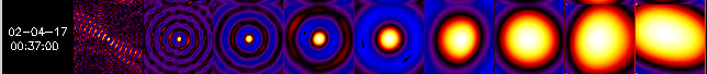
SC. In the following examples, there are 9 single-SC back-projection
maps shown side by side, with SC #1 the leftmost map and SC #9 the rightmost
one.
Example 1.
Example 2. 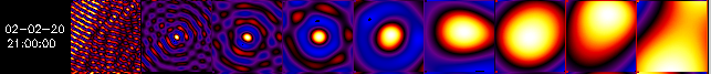
Example 3. 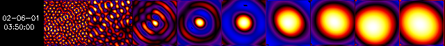
Example 4. 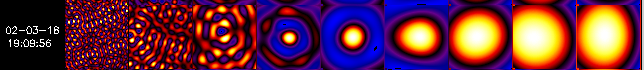
In Example 1, the back-projection maps for SC #1 through 9 show a clear single source with surrounding rings ("sidelobes") for all subcollimators. This means that you can use all detectors for mapping.
In Example 2, the first (SC #1) map shows nothing but stripes, while the SC #2 map shows the source as a dot surrounded by rings, and similarly for the SC #3 and SC#4 maps. So in this case, one would discard SC #1 and use SC #2 through 8 for mapping.
Example 3 shows a case where the SC #1 and SC #2 maps look like "wallpaper", but the SC #3 map shows a strong central source. Here you would use SC #3 through 9.
Example 4 shows maps where SC #1 though 3 give no central source,
indicating that the finest SC to use is #4.
Obviously the decision is more complicated for complex sources, but this
method works most of the time.
Generally, no. Don't bother using subcollimators with angular resolution greater than the size of the map. It adds little, if any, information. In fact, there is a danger of centroid skewing when using SC #9 if the map center is closer than 710" from the spin axis (which is true most of the time.)
For any subcollimator, when the map is closer than 2 angular pitches
(4 times the angular resolution), the centroid of the single-SC map will show
a significant shift, and this will skew a multi-SC map that includes that SC.
(In principle, this can be corrected for, but the current software doesn't
make any correction.)
First, the point spread function is available from an image object only when the 'CLEAN' algorithm has been used.
Assuming obj is a 'CLEAN' image object, type
psf_ptr = obj -> getdata(class_name='hsi_psf', /no_sum)
This will return a pointer array dimensioned (9,3) for 9 grids, 3 harmonics. Only the pointer array elements corresponding to enabled grids will be valid. Use ptr_valid (psf_ptr) to see which pointers are valid, and then dereference the one you're interested in.
For example,
print,ptr_valid(psf_ptr)
0 0 0 1 1 1 1 1 0
0 0 0 0 0 0 0 0 0
0 0 0 0 0 0 0 0 0
psf_grid4 = *psf_ptr[3,0]
Without the /no_sum keyword, the sum of the point spread functions for all enabled detectors is returned. Note that the point spread function is returned in annular sector units.
The algorithm that corrects for attenuator and decimation state changes looks for jumps in attenuator and/or decimation states *during the time interval selected*, and computes the correction from the count rates before and after the change in state. If the state changes more than once, during your selected time interval, then the correction factor is interpolated between the two state changes.
If you have a short time interval with just one attenuator and decimation state, it makes no corrections. If you extend it just a little to cross an attenuator state change, then the count rates are all normalized to the A1 state.
In the HSI_IMAGE and OSPEX objects, the plotman object reference is stored
internally. Every time you call
o-> plotman
it will add another panel to the same plotman interface. The
earlier plots are accessible under the Window_Control pulldown menu.
Unlike the image object, the HSI_SPECTRUM object does not store the plotman
object reference, so you have to do a little more. When you call the
plotman method, you can use the plotman_obj keyword. On the first call to
plotman, since the plotman object doesn't exist yet, a new plotman will be
created, and the variable reference will be returned. On subsequent calls,
new panels will be added to the existing plotman interface:
o-> plotman, plotman_obj=po ; first call, returns po
o->plotman, plotman_obj=po ; next call, uses po to add another
panel
If you are using the hessi GUI, you can retrieve the plotman object reference
via the hessi_data command (type hessi_data to get help on the command).
For example:
hessi_data,plotman=po
Then you can add plots to the GUI's plotman from objects that you have at the
command line, by using the plotman keyword to pass in that plotman object
reference:
o-> plotman, plotman_obj=po
In the hessi GUI, there's a button on the Imaging Widget under the Display pulldown button to plot the aspect solution for the time interval currently selected for imaging.
If img_obj is an image object then the following works:
img_obj->plot_aspect
img_obj->plot_aspect, /plot_triangle
asp_data = img_obj -> getdata(class='hsi_aspect_solution')
The aspect solution object can be retrieved from the image object via
asp_obj=img_obj->get(/obj,class='hsi_aspect_solution')
or created for a time interval via
asp_obj = hsi_aspect_solution(obs_time_interval='21-apr-2002 ' + ['00:45',
'00:46'])
Once you have an aspect solution object (called asp_obj) the following
works:
asp_obj -> plot ; this is the same plot as above
starting from the image object
asp_obj -> plot, /plot_triangle
spin_axes = asp_obj -> get_spin_axis() ; one pair of x,y coords per rotation
spin_axis = asp_obj -> get_spin_axis(/average, spin_period=spin_period)
print,spin_period
asp_data = asp_obj->getdata()
The asp_data structure returned by the call to getdata is described in the RHESSI Aspect Solution Users Guide.
See the previous question and use:
spin_axis = asp_obj -> get_spin_axis(/average, spin_period=spin_period)
The hessi spacecraft time format is a named structure (HESSI_SCTIME_FULL) with tags SECONDS and BMICRO. To convert to any of the standard anytim formats, use the hsi_sctime2any function with any of the keywords allowed in anytim. For example, the base time returned in the aspect solution structure, t0, is in spacecraft time format:
asp_data = asp_obj -> getdata()
print, hsi_sctime2any (asp_data.t0, /vms)
Last updated
16 May 2007
by
Kim Tolbert
,
301-286-3965