
This write up tells you a basic way to do spectral analysis of RHESSI data for a solar flare. Only spatially integrated spectra are covered here; imaging spectroscopy will be covered in a separate write up. I have chosen the X-class flare that occurred on 21 April 2002 as an example but the basic method can be applied to any flare. The steps necessary to carry out this analysis using the graphical user interfaces (GUIs) are described in detail but the same analysis can be carried out using the command line interface (CLI). An example scripts that can be run from the CLI can be found here and here. The user should first read Getting Started With RHESSI Data Analysis to ensure that the requirements for setting up IDL, the Solar Software (SSW) tree, and access to the RHESSI data have been satisfied before proceeding.
The procedure to do RHESSI spectral analysis requires two distinct steps with a data file and a spectrometer response matrix (srm) file as the interface between the two.
The first step involves reading the appropriate RHESSI data files and generating the count-rate spectra over a selected energy range for many time intervals spanning the flare, with additional intervals to allow the background spectrum to be estimated. At this stage, all corrections for live time, decimation, pulse pile-up, and energy calibration are taken care of. The output file contains the count-rate spectra in counts s-1 in the designated energy bins with uncertainties for all of the selected time intervals. A second file containing the spectrometer response matrix (srm) is also generated. The srm is the matrix of probabilities relating the measured pulse amplitude to the energy loss in the detector for all three states of the attenuator setting, A0 (no attenuators), A1 (thin attenuators), and A3 (thin plus thick attenuators). Note that attenuator state A2 (thick attenuators only) is not used in practice since it is so similar to A3.
The second step involves reading in the two files generated in the first step and generating photon flux spectra for each of the time intervals during the flare by the forward fitting technique. First, a method for determining the background in each interval is selected. Usually taking the rates before and/or after the flare is the easiest, but more sophisticated methods are often needed, especially if different attenuator states were used during the flare. In that case, the safest approach is often to use nighttime intervals before or after the flare. Next, the energy range to be used for the least-squares fit is selected and the functional form of the photon spectra is chosen. Starting parameters are determined to ensure that the fit is sufficiently close to the true minimum in chi-squared to allow convergence to the best-fit solution. The new OSPEX program is much more robust and forgiving than the old SPEX program so that this step is not so daunting as previously. The program will then automatically find the solution that minimizes the chi-squared value relating the observed background-subtracted count rate with the predicted count rate obtained by folding the assumed photon spectrum through the spectrometer response matrix. The parameters for this solution with their formal errors and other related information about each time interval are stored and can be saved in a file for future use.
The rest of this document is a case study, showing each step in the process using the two graphical user interfaces available for this purpose. The HESSI GUI (described in C:\ssw\hessi\doc\gui_help.htm) is used for step 1 and the OSPEX GUI (described in C:\ssw\packages\spex\doc\ospex_explanation.htm) is used for step 2. Script files can be generated by clicking on the "Write Script" buttons in each of these two GUIs, and they can be modified to carry out the complete operation automatically from the CLI. Examples of such scripts are available for Step 1 and Step 2.
Once IDL with access to the SSW routines has started type the following on the command line:
hessi
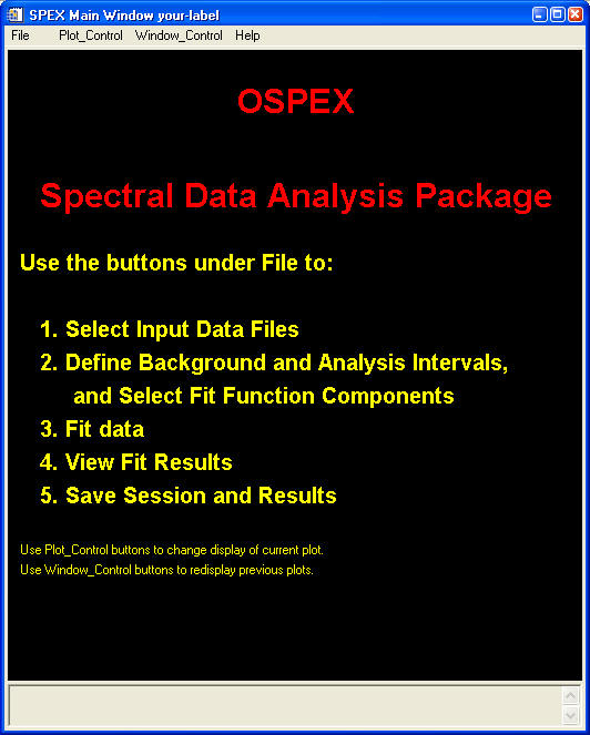
Depending on the speed of your computer the following window should open in about 10 seconds:
Next, as instructed in the center of this window, "Use the buttons under "File" to "Select Observation Time Interval..." A new window called Observation Time Interval Selection opens and after suitable editing of the start and end times should look as follows:

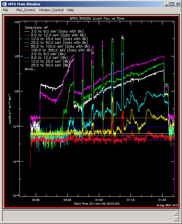
Clicking on the button marked "Plot Observing Summary Data" should get you the following plot in the main GUI window:
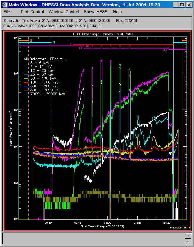
This is the standard time history for the flare of interest on 21 April 2002. Note that it is the summed counting rate of all the front and rear detector segments in counts s-1 detector-1. The detailed markings in this plot are described in detail in Kim Tolbert's write up on RHESSI Quicklook Light Curves The various changes in count rate with time in the different energy ranges are described in Brian Dennis' write up on Artifacts in RHESSI Light Curves.
This count rate plot gives us very important information on the impulsive phase of the flare of interest. We see, for example, that RHESSI came out of nighttime at about 00:33 UT as indicated by the vertical blue dashed line but more accurately, by the rapid increase in the 3 - 6 and 6 - 12 keV count rates. This indicates that a flare was already going on at this time. Images show that it was at a different location than the flare of interest that began at about 00:39 UT. (Note that right clicking on the plot gives you the time at the cursor.) The horizontal purple line at the top of the plot labeled A0 indicates that all attenuators were out of the detector fields of view at this time. The counting rate at all energies up to 25 keV rose very rapidly until at about 00:48 UT the thin attenuators moved into the detector fields of view (as indicated by the purple line dropping to the A1 level); the rates below 25 keV dropped precipitously at this time. Thereafter, every 4 minutes, the thin attenuators were removed for 1-minute intervals to test the low energy rate from the flare. At about 01:30 UT, the thick attenuators were added to the thin attenuators in the detector fields of view (the A3 state as indicated on the purple line) and the rates up to 50 keV dropped precipitously. Finally, at abut 01:33 UT, RHESSI went into night and the rates again fell to their non-solar background levels. Note that the rates up to 300 keV continued to climb as RHESSI entered the South Atlantic Anomaly (SAA) as indicated by the orange line marked with an "S" at the top of the plot. No data is recorded during passages through the most intense parts of the SAA to preserve space in the on-board memory.
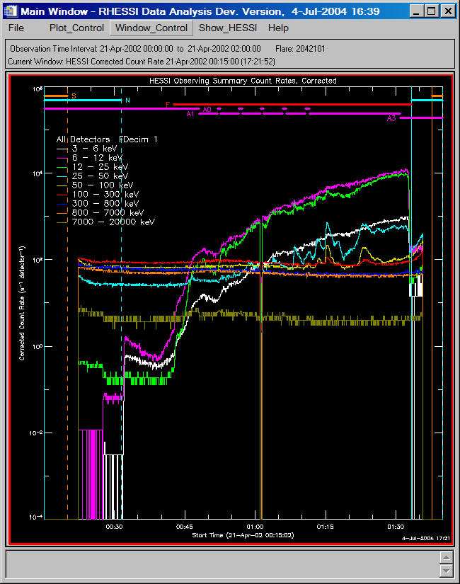
Note that you can plot several other things from the Observation Time Interval Selection window, perhaps the most useful of which is the "Corrected Count Rate." This removes the steps on the rate caused by the attenuator movements by simply multiplying the rates in the A0 and A3 states by the steps seen on going to or from the A1 state. Thus, the corrected count rates (shown below) are roughly what RHESSI would have counted if it had been in the A1 state the whole time.
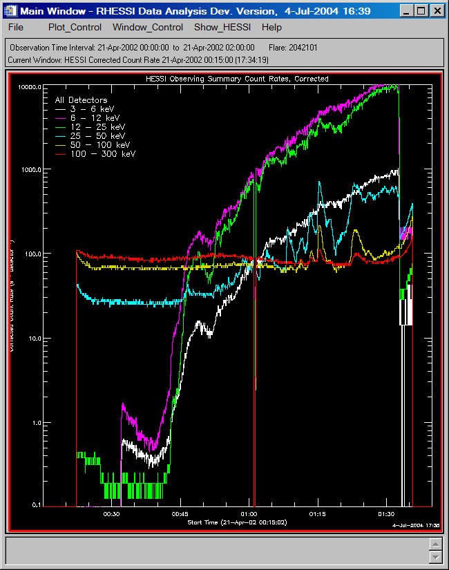
Note that any of the plots shown in the main GUI window can be reconfigured by using the very versatile "XY Display Options" in the "Plot_Control" menu. For example, you can just plot the corrected rates for channels up to 300 keV with all of the flags and indicator bars removed (using the "Change" option in the Observation Time Interval Selection window) as follows:
At this stage we can set the Observation Time Interval that we want and close the Observation Time Interval Selection widget by clicking on the "Set Obs time and Close" button.
Now we start the real spectral accumulation part of the exercise by selecting "Spectrum" from the "Retrieve/Process Data" option in the pull-down File menu of the GUI Main Window. This is where you will first access the full RHESSI data fits files. Thus, you must have access to the RHESSI data from one of the on-line servers or the files must be resident on your computer. If you have access to the internet, you can type
search_network,/enable
on the IDL command line to allow the HESSI GUI to search for the data files on the network. The data files will be copied into the directory returned by the environment variable HSI_DATA_USER defined in your setup.hessi.env file that you will find your in \ssw\site\setup directory.
The following "SPECTRA" window should now open:
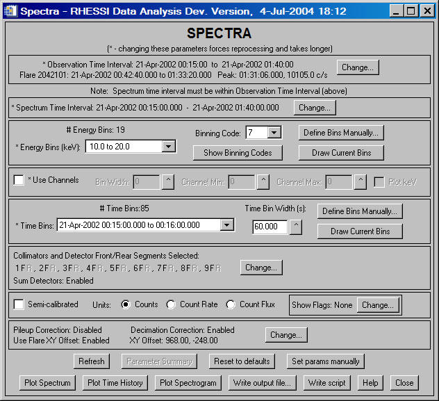
We want to change the energy bins, time bins, detectors used, and other options from the default values shown in this window.
First, we will change the energy bins. I prefer to use 1/3 keV bins for energies up to about 15 keV to give the best information on the iron and iron/nickel lines at ~6.7 and ~8 keV respectively. I use 1-keV wide bins from 15 to 100 keV and 5 keV bins up to 300 keV. For this event and most others, there are no counts above background for any higher energies. To set up these energy bins, click on the button labeled "Define Bins Manually..." There are several ways to set up the energy bins from the following "Select Energy Interval(s)" window that pops up.
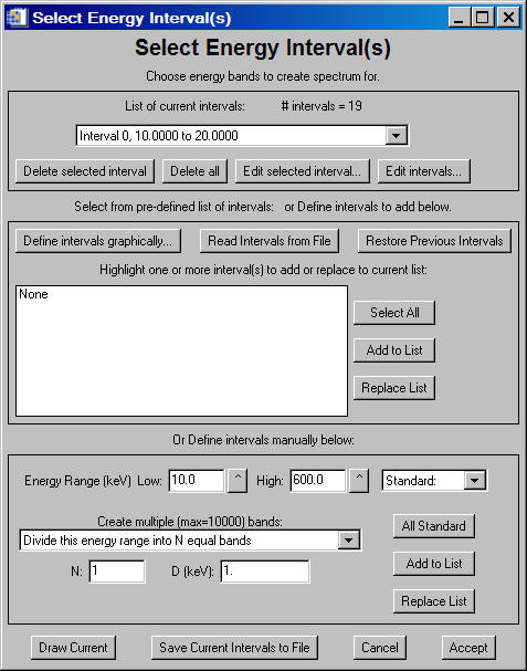
I prefer to use the "Or Define intervals manually below:" section of this window. Set the Energy Range (keV) Low:" to 3 keV by overwriting the 10.0 in the area next to this label. Set the "High" to 15.1 (to allow for round-off error?). In the drop-down menu under "Create multiple (max =10000) bands," select "Divide this energy range into bands of width D." In the area to the right of "D (keV)," type 0.33333333333. Then click on the "Replace List" button. You should see the "List of current intervals" near the top of the window show "# intervals = 36" and the drop-down list below this label should show 36 intervals from 3 keV to 15 keV, each 0.333 keV wide.
Next, set the "Energy Range (keV) Low" to 15.0, the "High" to 100.0, and "D (keV)" to 1.0. This time click on the "Add to List" button and see the "# intervals" increase to 121. Finally, set the "Energy Range (keV) Low" to 100.0, the "High" to 300.0, and "D (keV)" to 5.0. Click on the "Add to List" button and see the "# intervals" increase to 161. To avoid having to set these intervals up for each flare, click on the "Save Current Intervals to File" button near the bottom of the window. You will be asked for the name of a text file to save in your IDL working directory. I choose "energy_intervals_161.txt." Then the next time you want to use this combination of energy bins, you can just click on the button near the top of the window marked "Read Intervals from File."
Finally, click on the "Accept" button in the bottom right hand corner of the window and you will be returned to the "SPECTRA" window with your 161 energy bins.
Next, we must set up the time bins for spectral analysis. Note that you will be able to sum together the time bins chosen here in the section later where the actual spectral fits are calculated. The default time bins are 85 1-minute intervals spanning the selected "Spectrum Time Interval" shown near the top of the window. We want to change this to 4-s intervals spanning the same time range. The rational for this is that this is the shortest integration time for which the resulting count rates are independent of the rapid modulation produced by the grids as the spacecraft rotates. Strictly speaking, this time should be the rotation period of the spacecraft. The exact value of this can be determined from the plot of rotation rate vs. time given at this location. An ASCII version of this plot is available for more accurate determination of the mean daily spin period at this location.
Half the rotation period could also be used although there are minor differences in the modulation patterns for the odd and even rotations because of non-uniformities in the grids.
Generally, the nominal value of 15 rpm for the spin rate is accurate enough, especially if you will be integrating for longer periods for spectral analysis. For shorter time intervals, the different count rate modulation for the different detectors must be taken into account. This is now possible using Gordon Hurford's demodulator but it is not yet incorporated into the standard spectral analysis routines.
To set 4-s time bins, click on the button marked "Define Bins Manually" in the "Time Bins" section of the SPECTRA window. The "Select Time Interval(s)" window will pop up. This works similarly to the "Select Energy Interval(s)" window used previously. We choose to use the "Define intervals manually" section of this window. Notice that in the count rate vs. time plotted in the "Main Window" of the GUI, the data starts after exit from the SAA at 00:22:20 UT and ends on re-entry into the SAA at 01:35:42. Actually, the front segment data does not start until 00:27: 40 UT. The counts recorded at earlier times in this orbit are from the rear segments only. We will generate and save the count rate spectra starting in spacecraft night since we want to use the nighttime spectra as the background spectra when we can be sure that there was no solar contribution.
To select the full range of front segment data for this orbit, type 00:27:40 and 01:35:40 into the "Start" and "End" areas of the "Select Time Interval(s)" window, respectively. Note that the "Duration (s)" should then read 4402.000. Then we choose the "Divide this time range into intervals of length D" option from the "Create multiple (max = 100000) intervals" pull-down list, and set D = 4.0. Then we click on the "Replace List" button and "List of current intervals" area near the top of the window should show 1100 intervals. As with the energy bins, these can be saved in a text file by clicking on the button labeled "Save Current Intervals to File." I save the file called "time_intervals_1100x4s.txt" in a directory set up specifically for this flare. Finally, click on the "Accept button and the SPECTRA window should now show our 1100 time intervals each 4 s wide.
Next we must decide which detectors to use for the spectral analysis. The following considerations must be kept in mind in deciding this issue:
Since I am interested in resolving the iron and iron/nickel lines, I choose to use only the front segment of detector #4 to give the best possible energy resolution. I can repeat the analysis with the other individual detector front segments to give me independent results that allow me to determine the uncertainty on the spectral fit parameters. Alternately, I could choose more detector segments at this stage to improve the statistics in any one time interval. For this event, however, with the type of analysis I am interested in, count statistics is not a problem so I choose a single detector segment with the best energy resolution.
To select the detector segments to use, click on the "Change" button in the section of the SPECTRA window marked Collimators and Detector Front/Rear Segments Selected:" The following window will pop up:
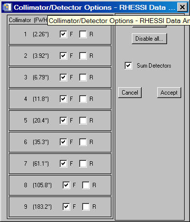
Click on the button marked "Disable all...:" and select "Front/Rear Segments" from the menu. Next click on the box labeled "F" next to Collimator 4 and note that it is checked. click the "Accept" button and note that all detector segment labels are greyed out except for "4F".
In the next section of the SPECTRA window, change the "Units:" to "Count Flux" so that the spectral plots will show counts cm-2 s-1 keV-1 fully corrected for detector dead time and data gaps.
The last thing we must decide is to enable or disable the pulse pile up and decimation corrections and the use of the XY offset of the source from Sun center. This is done by clicking on the appropriate "Change" button in lower part of the SPECTRA window. The following window will pop up:
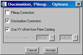
Note that the pileup correction is disabled by default. This is because it slows down the processing of the data considerably and is not needed unless the count rate exceeds ~1000 counts s-1 detector-1. However, for this flare the count rate exceeds this level for a considerable fraction of the time and the pulse pileup correction should be enabled. Note that if the rate exceeds ~100,000 counts s-1 detector-1 then the current pileup correction procedure does not do an adequate job since it does not consider more than two pulses piling up together. Thus, artifacts will still appear in the spectra at such high count rates.
Decimation correction is enabled by default and the count flux and statistical uncertainties automatically correct for the loss of photons below the decimation upper threshold energies.
The source XY offset from Sun center is taken by default from the values (in arcseconds) given in the RHESSI flare catalog that were obtained from the quick-look images . Different values can be entered if necessary by clicking on the checked box and typing in the X and Y values.
The SPECTRA window should now look like the following after you have made all of the changes from the default settings:
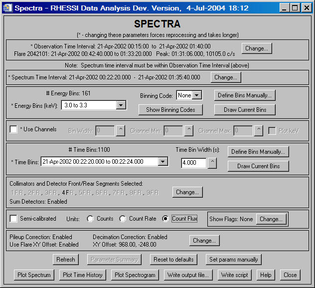
It's a good idea to write out the script to generate this state again without going through the GUI in case you want to repeat the same or similar analysis later. This is achieved by clicking on the "Write script" button
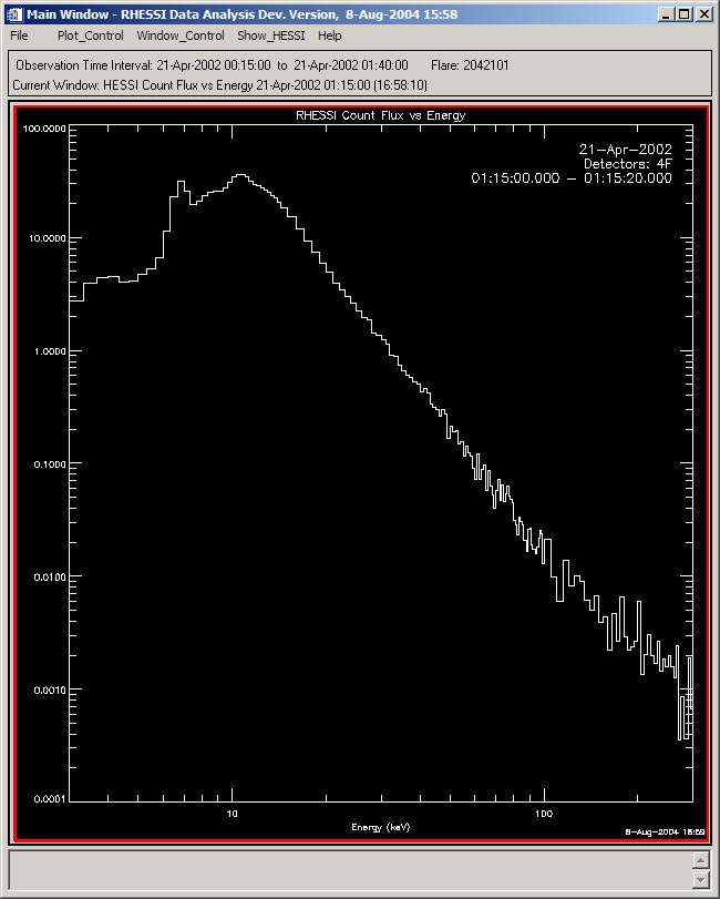
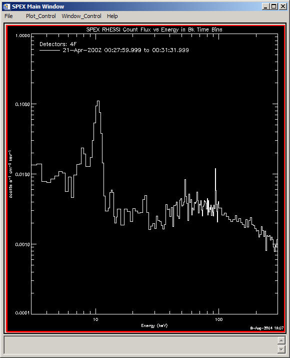
All that remains to accumulate the count flux spectra with your 161 energy bins and 1100 time bins is to click on the lower left button marked "Plot Spectrum." As a practical matter, it is usually a good idea to accumulate spectra for fewer time intervals to check that everything is set up correctly before you invest the considerable length of time that is required for the full time range you have selected. To do this go back to the "Select Time Interval(s)" window (click on the "Define Bins Manually..." button in the "Time bins" section of the SPECTRA window). Click on "Edit Intervals" and delete all but 5 or so intervals near the time of the peak of the flare - say at 01:15:00 UT - when you know that there should be good spectra.. Remember that you can always retrieve the 1100 intervals you set up earlier from the saved file. Click on the Accept button and note that the 5 intervals are now indicated in the SPECTRA window. Now click on the "Plot Spectrum" button to accumulate the count flux spectra for just these five time intervals and you should get the following plot (after moving the legend to the upper right via XY Plot Options under Plot Control):
If that was successful, you are ready to go for all 1100 time intervals so read them all back into the time bins from the saved .txt file and click on the "Plot Spectrum" button again.
Since this was a big flare with very high count rates, accumulating all 1100 spectra takes a little while since each count must be read individually from the telemetry file and placed in the correct bin. On my 1.8-GHz laptop with 512 MBytes of RAM, it took about 30 min. with the processor pretty much 100% busy all the time. Be patient and you should see this plot appear:
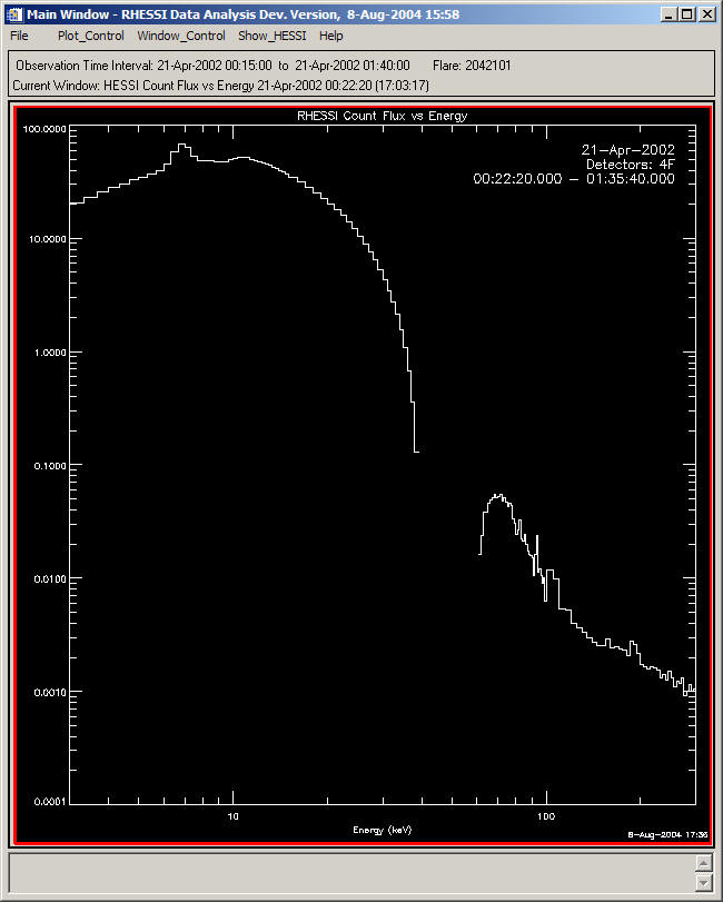
Don't be too alarmed at the shape of this spectrum. It is the spectrum for all time intervals added together and is dominated by the intervals when the attenuators were removed while the flux was very high. During those times, the count rates are higher than the pulse pileup correction algorithm is designed to handle, hence the distortion in the spectrum.
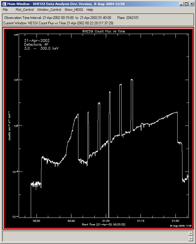
Click on the "Plot Time History" button and you should immediately see the following plot:
You are now ready to write the spectral data and spectrometer response matrixes out so that they are saved and can be read in by OSPEX or any other IDL procedure. Click on the "Write output file" button and see this window:
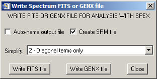
Change the option in the Simplify pull-down menu to "0 - Full calculation of diagonal, off-diagonal terms" so that the srm is used in all its glory instead of just the diagonal elements. Click on "Write FITS file" and select file names and locations for your data and the srm FITS files in the standard Explorer file selection window that appears. Give them unique names that tell you all the main attributes so that you will know how you generated them when you need to use them in OSPEX. I chose the following names with their sizes:
hsi_spectrum_20020421_002220_161ex1100i_d4_pu-enabled_8-8-2004.fits 2439 KB
hsi_srm_20020421_002220_d4_a013_pu-enabled.fits 386 KB
Note that the SRM FITS file contains the spectrometer response matrix for all the attenuator states that occurred during the time of data collection. Thus, in our case, it will contain all three matrixes for the A0, A1, and A3 states. OSPEX uses the correct version of the SRM for each time interval. OSPEX will not carry out any spectral analysis for intervals in which the attenuator state changes.
We are now ready to use OSPEX to analyze the count-rate spectra we just generated. If you have sufficient memory, it is most convenient to start a new version of IDL in a new window, leaving the GUI running in the old version.
To start OSPEX, type the following in the IDL command line:
obj=ospex()
Note that this defines an object called "obj" that OSPEX uses. You can call this object anything you like (within the IDL rules for naming objects) but you must remember the name if you want to extract anything from it or manipulate it from the command line. You can put various things inside the parentheses. One of the more useful is a label for the OSPEX window when it opens. You do this as follows where you can change your_label to whatever you want:
obj=ospex(gui_label = 'your_label')
After about 10 s, the following window should appear:
We will now go through the sequence of steps listed in this window to analyze the data file we just made in the GUI.
First, choose the "Select input" option from the File pull-down menu to get the following window:
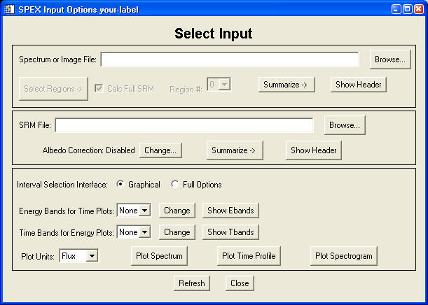
Click on the "Browse" button and find the Spectrum File that you just saved in the previous section. Once the correct path and file name appears in the "Spectrum File:" box, the correct path and file name should also appear in the "SRM File:" box, assuming you have not renamed or moved the files. The window should now appear as follows:

You can check to make sure you have the correct files by clicking on the "Summarize" buttons for each file and see the following information for the Spectrum file:
Spectrum or Image File Summary
File name: D:\My_Documents\My_HESSI\2002\04\21\Orbit1\spectra\OSPEX\hsi_spectrum_20020421_002220_161ex1100i_d4_pu-enabled_8-8-2004.fits
Data type: HESSI
# Time Bins: 1100 Time range: 21-Apr-2002 00:22:20.000 to 01:35:40.000
# Energy Bins: 161 Energy range: 3.00000 to 300.000
Area: 39.59
Detectors Used: 4F
Response Info: D:\My_Documents\My_HESSI\2002\04\21\Orbit1\spectra\OSPEX\hsi_srm_20020421_002220_d4_a013_pu-enabled.fits
and the following information for the SRM File:
Detector Response Matrix (DRM) File Summary
File name: D:\My_Documents\My_HESSI\2002\04\21\Orbit1\spectra\OSPEX\hsi_srm_20020421_002220_d4_a013_pu-enabled.fits
Data type: HESSI
# Count Energy Bins: 161 Energy range: 3.00000 to 300.000
# Photon Energy Bins: 177 Energy range: 3.00000 to 600.000
Geometric Area: 39.59
Separate Detectors: False
Detectors Used: 4F
Filter State(s): 0,1,3
You can then plot the count, rate, and/or flux spectra and time profiles to make sure they match what you obtained from the previous section. Here's what the flux time profile looks like:

This is similar to the summary time profiles we plotted in Step 1 but now only counts from the front segments are included so the background rates are lower and only data up to 300 keV are plotted. The energies default to the 9 standard RHESSI bands but you can choose different energy bands for the time plots by clicking on the "Change" button.
You can also plot the accumulated spectra and it should look the same as in Step1. Another option is a spectrogram, which, after adjusting the color table (click on "Image Colors" under "Plot_Control"), can be made to look as follows:

The vertical axis is energy in keV. Note the bright streak at ~6.7 keV during the flare from the Fe-line complex.
Now choose "Select Background" from the File pull-down menu to get the following window:
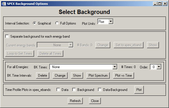
Since there are different attenuator states during this flare, the easiest choice is to select an interval during pre-flare nighttime period for the background. This gives an adequate background spectrum for our current purposes but may have to be refined for more detailed analysis in certain energy ranges and time intervals. Make sure that the "Order" is set to "0" so that the same background will be subtracted from all time intervals. Higher orders are used if more than one background interval can be used to define a polynomial for calculating a variable background.
Separate background time intervals can be selected in different energy bands if desired by clicking on the box marked "Separate background for each energy band.". The background energy bands default to the display energy bands set in the "Set Input" widget, but they can be changed if desired by clicking on the "Change" button.
To select a single background time interval, click on the "Change" button to get the following window to appear:

The light curve should simultaneously be plotted in the main OSPEX window. Left click on light curve at the start time of the desired background interval (~00:28 UT) and then right click on the end time (~00:31:30 UT). Click "Accept and Close" and you should see the background interval outlined on the light curves as follows:

Click on the "Plot Spectrum" button in the "Select Background" window to get the following plot:
Note the large peak from the germanium K-lines peaking at ~11 keV and other background lines above a smooth continuum.
To check that the background looks reasonable for different energy bands, check the "Data" and "Background" boxes at the bottom of the "Select Background" window to get the following light-curve plot with the background levels for each energy band:
If the background changes with time during the orbit, you can choose more than one background interval and fit the data with a higher order polynomial to give a better estimate of the background during the flare. Choose the order of the polynomial from the "Order:" pull-down option.
There is also the option to choose different background intervals in different energy bands for more difficult cases. To implement that option, click on the "Separate background for each energy band" check box. The SPEX Background Options window will transform to the following:
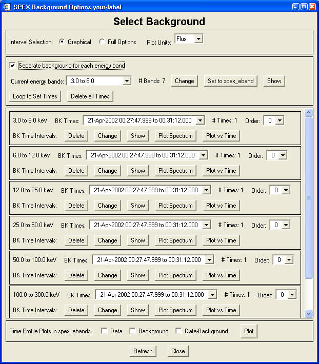
Click on the "Change" button for each energy band to select the time interval(s) in each case. Select the order of the polynomial in each case. Be sure to click on the "Plot vs Time" button for each energy band to make sure that the background estimates look reasonable.
Having satisfied yourself that the background estimates are acceptable in all energy bands, "Close" the "Select Background" window.
Now choose "Select Fit Options and Do Fit" from the "File" pull down menu in the main OSPEX window to produce the following window:

Here we must select the time intervals for analysis, the energy range to fit and details of how to loop through the intervals, one at a time.
We have the freedom at this stage to choose any intervals we like that are integer sums of the 4-s intervals we used when we made the spectrum data FITS files. Let us choose 20-s intervals covering the whole daytime part of the orbit. The easiest way to do this is to click on the "Change Fit intervals" button in the "Fit Options" window to produce the following:
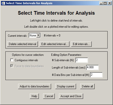
First, set "Length of Sub-intervals (sec)" to 20.000. Then left click on the start time at ~00:32:30 UT and right click on the end time at ~01:32:40 UT on the light curve in the main OSPEX window. Double left click in the resulting broad red band defining this period and select "Break into Sub-intervals of Equal Length (set in widget)" to produce ~180 intervals each 20-s long. Click on the """"Adjust to data boundaries" button to be sure that the time intervals start and end on the four-second interval boundaries. Finally, "Accept and Close" in the "Select Time Intervals for Analysis" window.
Click on the "Adjust Intervals" button and select the "Remove bad intervals completely" option to remove those intervals that include two different attenuator states, reducing the number to ~168 intervals. Finally, delete those intervals when the attenuator state changed from A1 to A0 for five brief periods since the counting rates were too high for the pulse pile-up correction to work. This can be most easily achieved by expanding the count flux vs. time plot to full screen , clicking on "Change Fit Intervals," then clicking on the bad intervals and selecting "Delete interval" from the "Edit intervals" menu that opens up. This leaves you with ~162 time intervals and the SPEX Fit Options window should look like this:

To set up the functions, energy ranges to fit and other fitting options, it is best to first choose an interval near the peak in the flare and loop backwards and forwards from there. Let's choose an Interval #117 that starts near 01:15 UT (just click on it in the "Fit Options" window) since we know that there is a hard X-ray peak at that time and the spectrum likely is made up of a well defined thermal (exponential) and nonthermal (power-law) components. Now click on the "Do Fit" button to produce the following window:

Here we want to define all of the functions that we expect to need to fit the data in each of the 168 time intervals we have defined. It is better to choose more functions rather than less since if you have to add a function later, OSPEX will delete all previous fits and start a new results file. You can see a full listing of all available functions by clicking on the "List" button. We will choose the following functions for this demonstration:
vth - Variable Thermal - the default
2 line - Gaussians for the iron-line complex peaking at ~6.7 keV and the iron-nickel complex peaking at ~8.0 keV.
bpow - Broken Power Law for the high energy nonthermal component.
First, select the "continuum" option in the "Keywords:" pull-down options list. Then add the above additional components one at a time. Note that you can see a description of a function and its adjustable parameters by clicking on its name once it has been added to the list.
Next we must set starting parameters for each function. The first thing to do is set the peak energy (2nd parameter) of the second line function to 8.0 and the integrated intensity (1st parameter) to 0.1 x the integrated intensity of the first line with the peak energy set by default to 6.7 keV line. Then click on "Plot All Components" at the bottom of the "Choose Fit Function Components and Set parameters" window to produce the following plot:
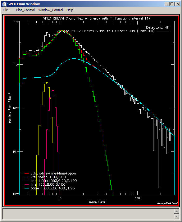
We see that both lines are too weak by about a factor of 100 so we can increase their a(0) values by this factor. The default values for the parameters of the other functions come acceptably close to fitting the data so that it is OK to try optimizing them by clicking on the "Fit" button. This produces the following two plots:


At this stage, we have a pretty good fit over the full energy range of the original spectral FITS file from 3 - 300 keV. The value for the reduced chi-squared is 1.65 (shown in the IDL window) and the plot of residuals normalized to one sigma shows reasonable values at energies above ~6 keV. We note that the attenuator state in this time interval was A1 so almost all the counts below ~6 keV suffer from K-escape and do not provide information about the incident photon spectrum at these low energies. We can eliminate these energies from the fitting by clicking on the "Change" button next to the "Energy range(s) to fit:" and typing "6.0 to 300.0" in the resulting XTEXTEDIT window.
We also note that there are peaks on the residual plot at ~7 and 9 keV. These can be reduced by allowing the peak energies of the two lines to be free. This is achieved by setting the appropriate number in the "Free" column to 1 for these to line energies. With these settings, we get the following (zoomed) spectra and residual plots:
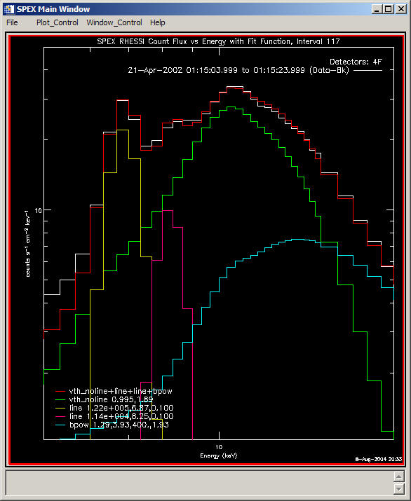
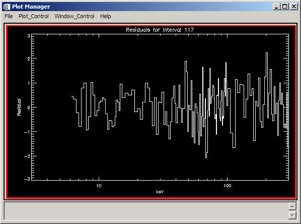
The value of chi-squared has been reduced to 0.69 and the residuals look more random. This is probably as good a fit as can be expected with the current accuracy in our knowledge of the SRM and background. The photon spectrum itself can be plotted as follows by checking the "Photons" box before clicking on the "Plot All Components" button:

One should be careful in interpreting the photon spectrum since it is well known that the data points tend to move towards the assumed spectrum with the forward fitting method used in OSPEX. More reliable spectra may be obtained with other forms of spectral fitting but this is beyond the scope of this demonstration.
We note that the chosen power-law function maintains the same slope of 3.93 down to the lowest energies. Hopefully, once we can use the information on the thermal plasma contained in the iron-line complexes, we should be able to better differentiate between the thermal and nonthermal components.
Once we are satisfied with the fit for this one interval, you should click on the "Accept" button to save the parameters and the spectra in the results file. This causes the program to refit the data and return to the "Fit Options" window. Here the count-rate and photon spectrum can be plotted with or without the background spectrum by choosing the appropriate options and clicking on the "Plot Spectrum in Fit Intervals" button.
Now we can set up the program to loop first forwards and then backwards through all the time intervals, starting with this one interval (#117) that we have just completed. The starting parameters for the different intervals can be set to equal the best-fit parameters from the previous interval, thus allowing them to be close to optimum. First choose all intervals from the one just analyzed forward to the last of the 20-s intervals in the "Fit Option" window (hold the shift key down while clicking on the last interval in the list). Make sure the "Loop Mode:" is set to "Manual First + Automatic" to allow you to check the fit on the first interval before allowing the program to attempt to fit all following intervals. The "Loop Direction" should be "Forward" and the "Param Init Method" should be "Previous Interval" before you click on the "Do Fit " button. in the "Choose Fit Function and Set Parameters" window, uncheck "Photons" to show the count rate spectra, and click on "Plot All Components" to make everything is as it was when you fitted the spectrum for this interval before. You can Click on the "Fit" button again to be sure but neither of these are necessary. Once you are certain that everything is set up correctly, click on the "Accept" button and the program should proceed to loop through all subsequent time intervals, attempting to obtain the best fit to the same functions you have chosen. You can watch the spectral fits appear for each interval to make sure they are reasonable or you can get a cup of coffee. It takes about 5-s per interval on my laptop. If something doesn't look right, you can always click on the "Cancel" button in the friendly "Progress Bar" that shows you what interval number is being analyzed and what best fit parameters are obtained.
Next you must analyze all the intervals from your starting interval (#117) backwards. This will be more difficult because early in the flare, there was no power-law extension to the spectrum and the counting rate was above the background only to energies as high as ~20 keV. Nevertheless, you can proceed bravely by selecting all time intervals from your initial interval back to the start. Set the "Loop Direction" to "Backwards" and click on the "Do Fit" button. This time, unless you suspect a problem, you can just click on the "Accept" button in the "Choose Fit Function and Set Parameters" window to let it loop backwards through all the preceding intervals.
Periodically, after completing various loops through the intervals, you should save your results. This is accomplished by choosing "Write Script and Fit Results" from the File drop-down menu on the main OSPEX window. You will have to choose file names and paths for the script file (default - ospex_script.pro) and the results file (default - ospex_results_8_Aug_2004.geny).
You can view the results by selecting "Plot Fit Results..." from the File drop-down menu. Displaying the different parameters as a function of time, adjusting the display in each case and plotting them from the Multi-Panel Options window (available from the "Window_Control" pull-down menu) results in the following plots:

Note the step in the thermal emission measure and temperature (parameters 0 and 1) at 01:31 UT after the thick shutters came in. Also, the dramatically lower temperatures before 00:43 UT like because of the decay of and earlier flare dominating the spectrum at these early times. The rise in the power-law flux at ~00:47 UT is caused by the high counting rates leading up to the thin shutters coming in.
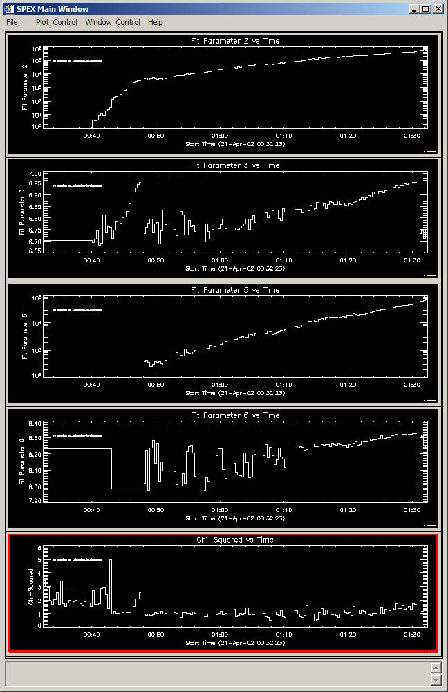
Note that the increases in the line energies at ~00:47 UT and from 01:20 - 01:30 UT are likely caused by the gain change as the count rates increased during these periods. The higher chi-squared values before ~00:43 UT resulted from the fitted energy range being changed to 3 - 15 keV and the likely presence of the decay of an earlier flare.
Further, more detailed, analysis of these fit results can be done by reading the output files into a separate IDL program as indicated in the Extracting Data from OSPEX.in Kim's OSPEX write up.