Table of Contents
We show, step by step, how to use the main features of the software.
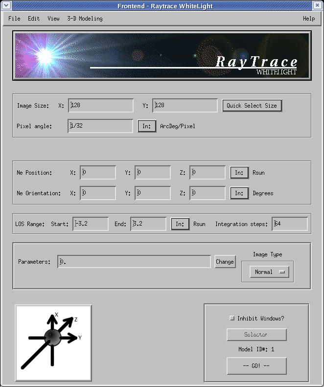
Run the rtfrontend. The window shown on figure Figure 4.1, “The Frontend.” should appear.
IDL[mycomputer]>rtfrontendFrom the menu → → →
Click on the pop-up parameter window.
Click the button and select .
In the LOS Range section edit the Start: and End: to respectively
-30and30.In the Parameters: section, click the button and select .
Check the Inhibit Windows? check box.
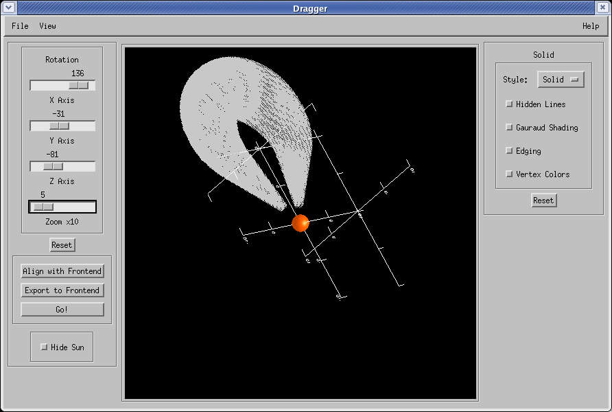
From the menu select . The Dragger window should appear (Figure 4.2, “The Dragger.”).
Now you can position the cloud model as you wish by clicking and dragging in the display area. Note that it's better if you zoom out a little bit down to 5.
Once you have positionned the structure the way you want, click on to generate the view. It can take few seconds.
Move the structure again so that it's viewed in a different position. Click on and then to generate the view. It can take few seconds.
Close the Dragger window.
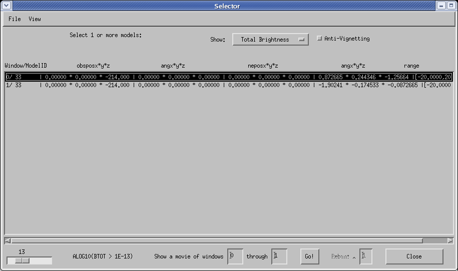
Open the selector window by clicking on (see Figure 4.3, “The Selector”).
Click on the image you want to display. The image is displayed in log scale. You can play on the cutoff using the slider on the botton left corner. You can also select if you want to visualize the , or .
You can generate a movie by clicking on .
The raytracing can be performed via the command line of IDL. It is of course less friendly than the front end but provide more flexibility if simulations need to be automated or included in a program. Three programs are implemented raytracewl, rtwlline and rtwlcirc. The first one generated images and the two other one radial and circular profiles.
The following examples show how to use the program in command lines. They also show different implemented features. For more details on the parameters and keywords, please refer to the header of the programs.
Example 4.1. Slab model simulation.
; -- simulation of a slab, edge-on
raytracewl,sbt1,sbp1,sne1,imsize=[256,256],losrange=[-30,30],$
losnbp=128L,modelid=14,neang=[0.,-39.5,-90-12]*!dtor,/c3,/fake
wnd,0,alog10(sbt1.im > 1e-14)

; -- simulation of a slab, face-on
raytracewl,sbt2,sbp2,sne2,imsize=[256,256],losrange=[-30,30],$
losnbp=128L,modelid=14,neang=[90.,-39.5,-90-12]*!dtor,/c3,/fake
wnd,1,alog10(sbt2.im > 1e-14)
- sbt1
Total brightness structures containing the image, the simulation parameters and a FITS header.
- sbp1
Polarized brightness structures containing the image, the simulation parameters and a FITS header.
- sne1
Integrated Ne structures containing the image, the simulation parameters and a FITS header.
- imsize
Size of the image in pixels.
- losrange
LOS integration range in R_Sun.
- losnbp
LOS number of integration points.
- modelid
ID of the model.
- neang
Rotation angles applied to the density model, in radian.
- /c3
LASCO C3 FOV preset.
- /fake
Create a fake LASCO FITS header.
Example 4.2. CME model simulation
raytracewl,sbt1,sbp1,sne1,imsize=[256,256],losrange=[-30,30],$$
losnbp=128L,modelid=33,modparam=[0.7,2.55,30.,10,.2],neang=[0.,-39.5,-90-12]*!dtor,/c3,/fake
wnd,0,alog10(sbt1.im > 1e-14)
- modparam
Parameters array corresponding to the model 33. See
models.cppfor details.
The model 26 is useful to perform raytracing through a user electron density cube. The format of the modparam parameter array is the following (see also the source code):
x size (sx)
y size (sy)
z size (sz)
xc Sun center in pix
yc Sun center in pix
zc Sun center in pix
![[Note]](note.png)
Note (0,0,0) is the center of the first voxel
voxel size in rsun, same for the 3 directions of space
data cube in lexicographical order (x,y,z)
We can build a fake electron density cube and make the raytracing for the example of it. Here it is a parallelopiped slab. Note that model 26 uses trilinear interpolation between neighbor voxels. For no interpolation, use model 25.
; ---- build the fake density cube
cube=fltarr(64,64,64)
cube[32:*,32:*,32:38]=1e4
; ---- build the parameter array
modparam=[64,64,64,32,32,32,0.8,reform(cube,64L*64L*64L)]
; ---- generate the view
raytracewl,sbt,imsize=[256,256],losnbp=64L,losrange=[-20,20],$$
modelid=26,modparam=modparam,neang=[90,-80,30]*!dtor,/cor2
This model (#4) uses density cube from Y.-M Wang potential field source surface extrapolation program. In that example, a default density cube for the CR 1926 is downloaded, so that the parameters are hidden in the command line but appended within the program (see the source code). The simulation is done with a LASCO C1 FOV.
raytracewl,sbt,imsize=[256,256],losnbp=128L,losrange=[-2,2],$$
modelid=4,neang=[0,90,0.]*!dtor,/c1
wnd,0,alog10(sbt.im > 1e-9)
In the model 11 a map of the neutral line position is passed to the program. The corona is filled of electron density according to the distance of a given point to the neutral line. It is useful to reproduce, on average, the streamer belt.
; ---- download the CR2012 SSFM from WSO
rdtxtmagmap,nsheetmap,crot=2012
; ---- format parameter array in single row vector
modparam=reform(nsheetmap,n_elements(nsheetmap))
; ---- run raytracing
raytracewl,sbt,imsize=[256,256],losnbp=64L,losrange=[-20,20],modelid=11,modparam=modparam,neang=[0,90,0.]*!dtor,/cor2
; ---- display total brightness
wnd,0,alog10(sbt.im > 1e-14)
For the example, use the CME model simulation. The extra-parameter rho output the impact parameter, the distance between the LOS and the Sun center.
raytracewl,sbt1,sbp1,sne1,imsize=[256,256],losrange=[-30,30],$$
losnbp=128L,modelid=33,modparam=[0.7,2.55,30.,10,.2],neang=[0.,-39.5,-90-12]*!dtor,/c3,/fake,rho=rho
wnd,0,alog10(sbt1.im > 1e-14)
oplotimpactgrid,rho,levels=[1,(findgen(7)+2)*4],$$
c_labels=replicate(1,10),ystyle=5,xstyle=5,c_linestyle=1
Radial profile along the slab model, edge-on.
rtwlline,sbt1,sbp1,sne1,imsize=[512,512],losrange=[-30,30],$$
losnbp=256L,modelid=14,neang=[90.,-39.5,-90-12]*!dtor,/c3,/fake,$$
angle=-39.5*!dtor,nbpix=250L
plot,sbt1.im,/ylog,yrange=[1e-13,1e-8]
- angle
Polar angle of the profile. Remember that in the raytracing software basis the X axis is upward, the Y axis toward right and the Z axis points from the image plane toward the inside of the display.
- nbpix
Number of pixel for the profile. The pixel 0 is always at the center of the Sun.
Circular profile along the slab model, face-on.
rtwlcirc,sbt1,sbp1,sne1,imsize=[512,512],losrange=[-30,30],$$
losnbp=256L,modelid=14,neang=[0.,-39.5,-90-12]*!dtor,/c3,/fake,$$
radius=100,nbang=360L
plot,shift(sbt1.im,90),/ylog,yrange=[1e-15,1e-12]
- radius
Radius of the circular profile in pixel. The center is at the center of the Sun.
- nbang
Number of pixel for the profile. 360 pixels makes 1 pixel per degree.
buildcloud generates a density cube for a given model. The cube is saved in a text file and is formated for the Dragger visualization tool. The following example shows how to build a density cube for the model 14. It creates a 64 x 64 x 64 cube of 60 x 60 x 60 R_Sun, the Sun center being at the center of the cube.
buildcloud,14,cubesidenbpix=64L,cubesidersun=60.