Table of Contents
We can define two types of model representations: geometric function and density cube. The octree compression and voxel list are extensions of the density cube representation.
The model is defined by a geometric function that gives the electron density for a given position x,y,z in space. The geometric function generally will have some extra parameters in order to be able modify the geometrical aspect of the model.
The electron density is given by a three-dimensional density cube. Each voxel of the cube contains a sampled value of the electron density at a point of the space. The cube can be either regularly or irregularly gridded. The advantage of the density cube is that it can contain the representation of a complex structure than would not be possible to describe simply with a geometrical function. On the other hand, if a fine resolution is needed in order to represent the fine details of a coronal structure for example, the storage size of the density cube can be a limitation. The storage size varies with the cube of the resolution. To double the resolution  times more memory is necessary. Note that density cube is generally the format used to store the product of a tomographic or stereo view inversion program.
The octree compression is a method use to compress the size required to store a density cube. It can be compared to the quadtree compression for a two dimensional image. If between 4 contiguous voxels of the cube the density variation is small enough, the octree compression consist in merging these 4 voxels in one single super voxel, containing then only one electron density sample instead of 4. This compression is very efficient when large area of the space are empty, when a cube contains a localized coronal structure for example. For descritions and application of octree compression see [1997adass...6..230V]. Algorithm for fast rendering of octree compressed cubes also exist (CITE)
The K corona is an ionized gas so roughly half of the particles present in this gas are free electrons. These electron are accelerated by electromagnetic field passing through the corona. As a result, they will scatter the solar light. This is because of this process that we see the corona in white-light. It is defined as the Thomson scattering. Note that light scattered by this process is polarized. (MINAERT, VAN DE HULST, BILLINGS) treated the problem of Thomson scattering in the solar corona. They established two equations that give the total and polarized brightness scattered from the solar photosphere by a localized electron density. It allows to calculate the brightness of the corona as seen from a telescope if we integrate along the lines of sight of this telescope. The Solar Corona Ray-Tracing program (SCoRT) is an implementation of these equations.
There are two methods to perform numerically the raytracing: ray-casting and splating. The choice of the method depends on the type of model we need to simulate: geometric function or density cube. Both methods have advantage and inconvenient. Processing speed is the major factor that will govern the choice.
At each pixel of the image corresponds a line of sight (LOS). For each pixel of the image we scan the space along the corresponding LOS. At each point of the LOS we get the electron density of the model and calculate the Thomson scattering geometric factor in order to get the corresponding brightness scattered by the electron density at that point of the space. Finally, the pixel value is the sum of all the contributions along the LOS.
Ray-casting is used for geometric model rendering. The major problem is that the program scan all the space (actually the space delimited by the user's boundaries) and can waste processing time where the space is empty if the model structure is localized. Adaptative step integration can be used though to speed up the rendering. Processing speed also mainly depend on the complexity of the geometric function. In some cases, the computation of a density cube could be suitable first and then render the cube on a second stage, eventhough we would lose the advantage of the geometric function which allows to change the model parameters for each rendering.
Splatting is particularly suitable for density cube rendering. We calculate the projected area of a density cube voxel on the image (instrument virtual CCD). This projection can be considered as the "shadow" of the voxel on the image. Then we scan the image pixels covered by the projection of the voxel. For each of the pixel we calculate the Thomson scattering geometric factor corresponding to the middle point of the LOS passing through the voxel. Then the scattered brightness is calculated and added to the pixel. We proceed voxel by voxel so that the final image is the sum of all the voxel contribution.
![[Note]](note.png) | Note |
|---|---|
Octree compressed density cube and voxel list could be rendered as well using this method eventhough performances can be increased especially in the case of octree compressed cubes (CITE REFERENCES). |
| Note |
|---|---|
Density cube can also be rendered with ray-casting method. In that case for each point of the LOSes an interpolation is performed to obtain the density at that point of the space depending on the density of the nearest neighbor voxels of the density cube. This rendering method can be useful if we set a coarse LOS step to get a quick first overview of the cube. |
All the coordinate systems are direct and orthonormals. Figure Figure 2.1, “Coordinate systems.” shows a summary of the 3 coordinate systems described in this section.
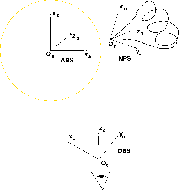
This is the coordinate system that is the reference for all the other systems described bellow: translation and rotation of the other coordinate systems will be calculated with respect to this one. The origin is at the center of the Sun.
Defines the position and orientation of the observer with respect to the absolute coordinate system. We use the optics convention for the axis of the virtual imaging telescope:
- Ox
Vertical axis of the CCD camera.
- Oy
Horizontal axis of the CCD camera.
- Oz
Optical axis of the telescope.
Defines the position and orientation of the electron density cube or model with respect to the absolute coordinate system.