Click here to see the entire HESSI GUI Guide
The HESSI Spectrum Widget is a graphical interface to the HESSI spectrum object. The object and the interface are connected closely; the interface provides an easy way to set parameters in the object and call the process method of the object to generate a spectrum.
The Spectral Executive (SPEX) package developed by Richard Schwartz is used to analyze HESSI spectra. Access to SPEX through the HESSI GUI is under development. As of October 2001, you must store the spectra in either a FITS file or a GENX file and then use that file as input to the SPEX program outside of the GUI. SPEX provides a uniform interface suitable for the X-ray spectral analysis of a number of solar (or other) instruments in the X and Gamma Ray energy ranges.
This widget is activated when you click File / 'Retrieve/Process Data' / Spectrum in the Main GUI Window. The overall time interval of the spectra you generate is constrained to be within the Observation Time Interval selected in the Main GUI.
When you first enter the Spectrum Widget, the spectrum parameters are set to the generic spectrum defaults, except for the time interval which is set to the observation time interval you selected.
When you change any of the spectrum parameters, they are set in the spectrum object, and are remembered the next time you enter the spectrum widget. Note: even if you select a new flare, the spectrum parameters are not set to defaults, but are remembered as you last set them (except for the time interval). You can reset the parameters to defaults by clicking the 'Reset to defaults' button.
Refer to the Overview of the HESSI Command Line Interface for a complete description of the spectrum parameters. Below is a cross-reference table showing the object control parameter names corresponding to the names in the widgets.
Selecting Time Interval
To select the overall time interval over which the spectrum will be made, click the Time Interval Change button on the Spectrum Widget. The time interval must be contained within the observation time interval you have selected. (Use the Time Bin Width to define time bins for the spectrum.)
Selecting Energy Bands
In the energy binning box in the Spectrum Widget, the droplist showing the current energy bands is only for display. You can not use the droplist to set energy bands. There are two methods for setting the energy bands:
- Select one of the pre-defined binning schemes by selecting a binning code. Click here for a list of what the codes mean.
- Define energy bins manually. The bin selection widget lets you graphically define bins, or manually edit a list of energy bins. You must plot a spectrum first. Click here for instructions on using the interval selection widget.
The 'Show Current Bins' button will draw the current bins on the spectrum plot if a spectrum plot is displayed.
Selecting Time Bins
There are two methods for setting the time bins:
- Enter a time bin width in seconds.
- Click 'Define Bins Manually' to graphically define time bins or manually edit a list of time bins. You must display a time plot (of any kind) first. Click here for instructions on using the interval selection widget.
The 'Show Current Bins' button will draw the current bins on the time plot if a time plot is displayed.
Selecting Collimators
To change collimator options, click the Change button in the collimator box.
Currently the collimators are always summed. To plot collimators separately, you must select and plot them individually.
Selecting Semi-calibrated Data
Semi-calibrated data includes the effects of detector efficiency, attenuator state, and grid transmission (spin-averaged, not time-resolved). The units are photons cm-2 s-1 keV-1. If the button to use semi-calibrated data is not set, then the units of the data are counts cm-2 s-1 keV-1.
Click 'Plot Spectrum' to accumulate and plot the spectrum. Click 'Plot Time Profile' to plot the time profile. Once plotted, use the XY Plot Display Options under the Plot_Control pull-down menu in the main GUI to alter the display. For example, the XY Plot Display Options widget lets you plot the time intervals used in the spectrum as separate traces instead of summing them.
Each plot that you create is saved as a plot panel in the main HESSI GUI,
called
HESSI Spectrum dd-mmm-yyyy hh:mm:ss (HH:MM:SS) or
HESSI Flux vs Time dd-mmm-yyyy hh:mm:ss (HH:MM:SS)
where dd-mmm-yyyy hh:mm:ss is the start time of the data in the plot, and (HH:MM:SS)
is the time you generated the plot. You can restore these plots or display
multiple plots simultaneously by using the
Window_Control
pull-down menu in the main GUI.
In order to analyze the HESSI spectra, you must write either a FITS or GENX file to pass into the SPEX program. FITS and GENX files contain the same information in different formats. Once the file is read in SPEX, the spectral analysis results will be the same regardless of whether a FITS or GENX file was used. The only basis for choosing is your personal preference. The FITS file follows the FITS RATES standard, and is readable by generic FITS readers. The GENX file can be restored in an IDL session using the restgenx SSW routine. Another consideration is that the FITS file may be ~4 times larger than the GENX file.
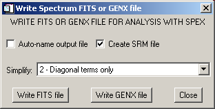
When you click the 'Write Output File' button, the following widget appears:
SPEX requires a Spectral Response Matrix (SRM) File in order to deconvolve the spectrum. Choosing to write the Spectral Response Matrix (SRM) File while writing the FITS or GENX file will ensure that you have the most accurate response matrix for your spectrum. Computing the SRM is time consuming though, so if you don't need the accuracy, in SPEX you can use an existing HESSI SRM file computed for a different time.
The options in the Simplify pulldown menu apply only if you enable 'Create SRM File'. The Simplify options dictate how the matrix will be computed. The options are:
Note: The FITS/GENX widget is a 'modal' widget, which means that you can interact only with this widget until you close it (you can't type anything at the command line or click in any other widget).
Table 1. Spectrum Widget Names Cross-Referenced to Object Parameter Names
| Widget Name | Object Parameter Name |
| Spectrum Time Interval | obs_time_interval, time_range |
| Energy Bins | sp_energy_binning |
| Time Bins | sp_time_interval |
| Collimator | seg_index_mask |
| Sum Detectors | sum_flag |
| Use Semi-calibrated Data | sp_semi_calibrated |
| Code | # bins | Description |
| 0 | 3 bins | Three energy bands, 10 keV wide, starting from 20 keV. Used mostly for quick software checks, but it could be useful for some hard x-ray work. |
| 1 | 99 bins | 1-keV bands, covering 1 to 100 keV. Possibly good for high-resolution hard-x-ray work (fitting thermal and nonthermal emission, etc.) |
| 2 | 5 bins | The three bands from "0" plus 50-100 and 100-200 keV bands; we will probably use this binning for a lot of non-solar work with the rear segments. |
| 3 | 7 bins | A broad band from 20 to 200 keV followed by 6 narrow bands (4-keV wide) to 224 keV. Used in software debugging. |
| 4 | 1000 bins | 1-keV bands from 3 to 1003 keV. Mostly useful for generating finely-detailed response matrices for debugging and display purposes. |
| 5 | 565 bins | 1-keV each up to 100 keV, then 5-keV bands to 1820 keV, and 10-keV to 2500. In addition, there are sections of fine binning around the 511 keV and 2.2 MeV lines. This is a good choice for first-look spectroscopy of gamma-ray flares. |
| 6 | 199 bins | 1-keV bands covering 1 to 100 keV, then 5-keV bands to 600 keV. A more complete binning than "1" for studying hard x-ray continuum spectra out to higher energies. |
| 7 | 19 bins | 10-keV bands from 10 to 100 keV, then 50-keV bands to 600 keV. Good for survey work to select spectra for closer analysis with "6". |
| 8 | 78 bins | 3-keV bands from 1 to 118 keV, then 15-keV bands up to 703 keV. Intermediate between "6" and "8" in memory use for hard x-ray work. |
| 9 | 4 bins | 12-keV bands from 200 to 248 keV. Another debugging mode. |
| 10 | 9 bins | Pseudo-logarithmic binning covering the entire HESSI energy range. The bin edges are at [3, 6, 12, 25, 50, 100, 300, 1000, 2500, 20000] keV. These spectra should contain all the events in the HESSI data stream (minus any rejected by event selection criteria like segment choices or coincidence rejection). Potentially useful for quick screening to separate x-ray from gamma-ray flares, etc. |
Last updated 07 November, 2008 by Kim Tolbert , 301-286-3965