RHESSI Imaging - First Steps
Last updated: 01-Jul-2005
This is a beginner's guide to RHESSI imaging using the RHESSI Graphical User Interface (GUI). It assumes that your computer has already been set up to run IDL with the solar software tree (SSW) and access to the RHESSI data (see Software Installation Instructions and Accessing RHESSI Data). To learn about RHESSI imaging using the IDL command line, see An Overview of the Command Line Interface. Imaging spectroscopy is not covered in this demonstration; further analysis is required to obtain spectra for different areas within an image. See Spectroscopy-First Steps for a demonstration of how to obtain spectra. For more details on RHESSI software refer to the RHESSI data and software center.
For this demonstration, we have chosen a flare that occurred on February 20 at 11:00 UT. We demonstrate how to obtain a quicklook light curve plot for this flare, and an image for the energy interval of 12-25 keV for 4 seconds at the peak of the flare.
To get started, enter an SSW IDL session and type hessi on the IDL command line.
Selecting a Flare Time Interval
First we'll take a look at the time profile of the flare. This is not required for making an image, but is recommended so that you can check the status of various indicators (e.g. day/night, attenuator state, SAA) and check the energy ranges in which the flare can be seen. We'll use the observing summary data (pre-binned to 4-second intervals, 9 energy bands) since it's quick. To see a time profile at different time/energy resolution we could use the lightcurve or spectrum interface (Creating a Light Curve or Spectroscopy-First Steps), but that's usually not necessary at this point.
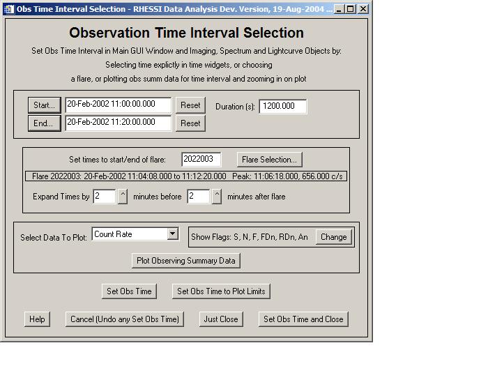
Click the “File” pull-down button in the Hessi GUI and choose “Select Observation Time Interval”. This will open a new widget.
Select start and end times. Type your times
directly into the text boxes, or click “Start” or "End"
and enter the date and time chosen for the demonstration: 20-Feb-2002 11:00:00
to 11:20:00. Another way of selecting a flare time interval is
to enter the flare number next to “Flare Selection". The flare number
for this flare is 2022003. Next
to “Duration” type in “1200”. This will change the end time to
1200 seconds after the start time.
Click “Plot Observing Summary Data”. This will generate a quicklook light curve plot showing count rate vs. time in the main window.
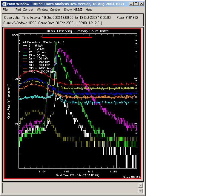
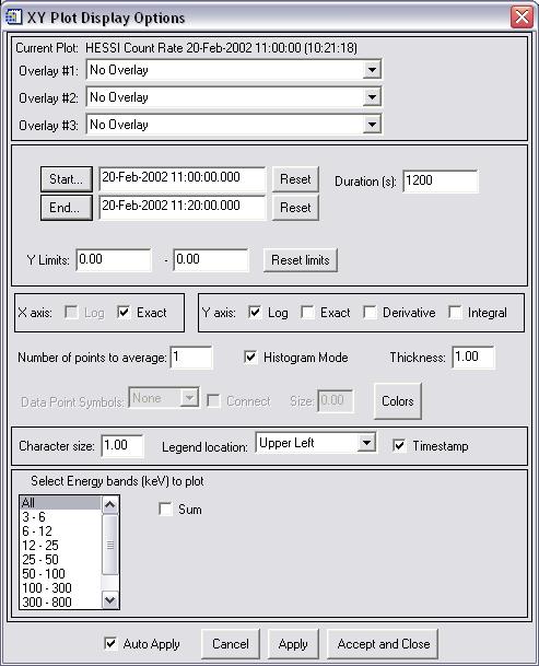
We can zoom in on this plot by left-clicking and dragging (a single left-click will unzoom). Or we can customize the plot by clicking "Plot_Control" and then selecting "XY Plot Display Options". The following widget pops up. Select each energy band in turn to clearly see the time profile in each energy range.
From these plots we can see that the front decimation state and the
attenuator state were both 1 for the entire flare (that's what the FDecim 1
and Att 1 mean), there is no night or SAA (South Atlantic Anomaly)
interval to worry about, and the flare is visible between 6 - 50 keV.
We'll choose the energy band 12-25 keV in the next section to create an image.
Refer to Artifacts
in RHESSI Light Curves to learn how to interpret a light curve.
Note that through the "Observation Time Interval
Selection" interface, we could also examine the
Ephemeris, Modulation Variance, or other quantities for this time interval by
clicking in the "Data Type" pull-down menu. Also, we can choose
which flags to display on the time plots, such as day/night, SAA, decimation and attenuator state by clicking the "Change"
button next to "Show Flags".
Click "Set Obs Time and Close".
Making an Image
Now we'll create an image using the 12-25 keV energy band for 4 seconds at the
peak of this flare. Click
the “File” pull-down button on the main GUI window, and click “Retrieve/Process Data”, and
“Image”. The Imaging widget will appear:
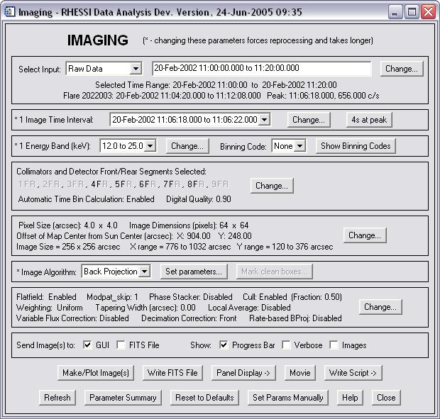
Note that the image time interval
defaults to the 4 seconds at the peak of the flare, and the energy band defaults
to 12-25 keV. We could change these by clicking the appropriate "Change"
button, but for our example, we don't need to.
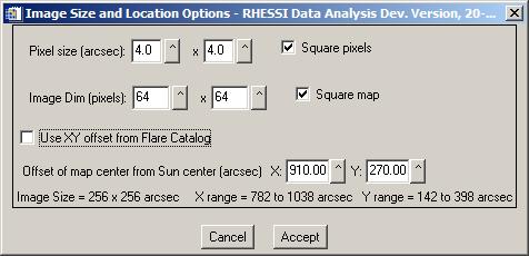
The default location of the flare on the Sun is retrieved from the online RHESSI Flare Catalog. In most cases this value can be used, but in some cases it may be 0.,0. or may be wrong. Follow the Separate Instructions for finding the flare location if you need to determine it yourself. In this example, we'll use the results of those instructions. Click “Change” next to "Offset of Map from Sun Center". Uncheck "Use XY offset from Flare Catalog" and type in 910. for “X” and 270. for “Y”. We'll accept the defaults for 4 x 4 arcsec pixel size, and image dimensions of 64 x 64 pixels, which will give us an image of 256 x 256 arcsec.
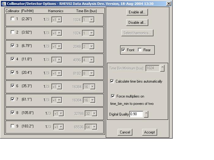
We want to use detectors 3-8, front segments for our example. Click “Change” to select these collimators if they are not already selected and make sure that “Front” is selected and "Rear" is not selected. For guidance on which detectors to choose, refer to "How do I determine which subcollimators to use when making a map?" in the RHESSI FAQ.
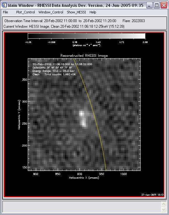
Next to “Image Algorithm”, the “Back Projection” reconstruction process should already be selected. Next to "Send Image(s) to" the "GUI" box should be checked. Click “Make/Plot Image(s)” and in a minute or two you will see the image:
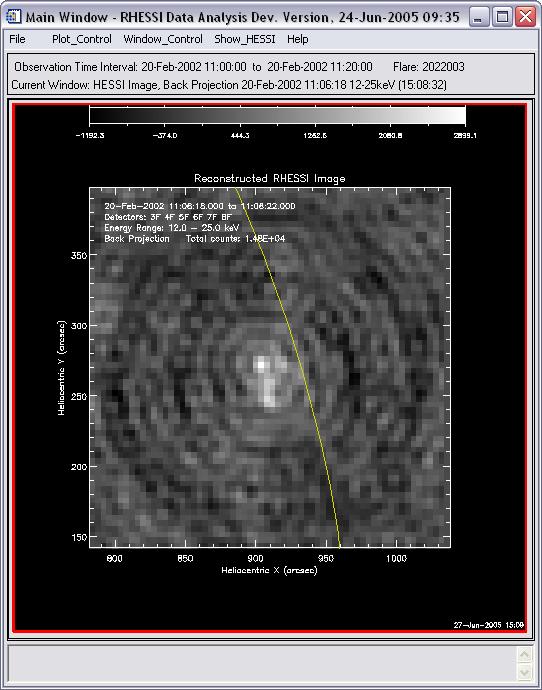
The yellow arc across the image
shows the position of the Sun's limb.
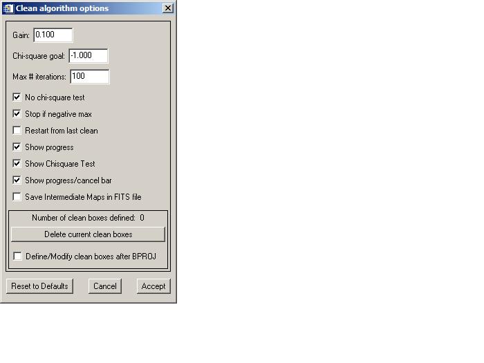
The rings around the bright source are side lobes. You can remove them by changing the "Image Algorithm" to "Clean" in the "Imaging" widget. After selecting "Clean", click "Set Parameters" and a "Clean algorithm options" widget will pop up. Change the "Max # iterations" to 100 and click "Accept". Click "Make/Plot Image(s)" again and a CLEAN image will be generated. Since the "Show progress" option was set by default (in the "Clean algorithm options" widget), an HSI CLEAN plot window will appear showing the iterations in the CLEAN algorithm as it works to remove the side lobes and create a cleaned image.
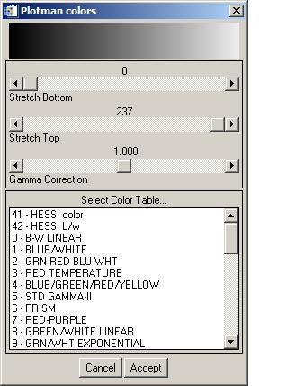
You can make this image a
different color by clicking on the "Plot
Control" pull-down button and selecting "Image Colors". Select "Hessi color" and
click "Accept".
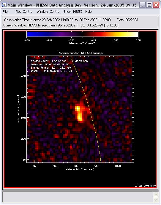
In this image you can begin to see the double-source nature of this flare that has made it so interesting to analyze. You can still see some arcs of circles centered on the location of the spin axis that indicate discrepancies in the flat-fielding process and in the point-spread functions that are used in the CLEAN process.
This completes the demonstration of the basic technique for obtaining RHESSI images. Now that you have been through the basic steps, you can try to refine the image by choosing different detectors, changing the pixel size, using different time intervals, and using one of the other image reconstruction techniques - a Maximum Entropy Method (MEM Sato or MEM VIS), Pixon, or Forward Fitting. Be aware that only Clean and Pixon give reliable results currently, and Pixon can take hours to complete. You can also make images for multiple energy ranges and multiple time intervals and view them as a movie, or use them for further analysis via imaging spectroscopy. For more complete information about the options in the Imaging widget see HESSI Image Widget.
Note that all of the plots made in any GUI session are available for the duration of that session. You can find them under "Window_Control" in the main GUI window. You can also save plots in PS, PNG, TIFF, or JPEG format by clicking "Create Plot File" under the "File" pull-down menu.
Last updated: 01-Jul-2005