RHESSI Spectrum Software
| On this page: | External Links:
|
RHESSI Spectrum Software Basics
The RHESSI spectrum software can be used from the IDL command line or the RHESSI GUI. A useful guide to accumulating a spectrum from the command line or the GUI is here.
The spectrum software starts with an hsi_spectrum object. By setting parameters in the spectrum object, you control the spectrum accumulation.
The spectrum control and info parameters are listed in the Spectrum Object Parameter Table. The control parameters most commonly set in the spectrum object by users are as follows (control parameter name in parentheses). Look in the table for more description of each parameter.
- time intervals (obs_time_interval, time_range, sp_time_interval)
- energy bins (sp_energy_binning)
- detector segment selection (seg_index_mask)
- front segment decimation correction (decimation_correct)
- rear segment decimation correction (rear_decimation_correct)
- data units (sp_data_unit)
- structure or array returned by getdata (sp_data_struct)
- separate detectors or combined (sum_flag)
To make a spectrum from the command line, you create a spectrum object, set your options, and request the data. As with all the RHESSI objects, all of the parameters are set to default values (shown in the parameter table, or by typing print,o->get(/xxx)) and you need to set only the values that you want to change. The only parameter for which there is no valid default is the time interval - you must set the obs_time_interval and/or sp_time_interval parameter. For example,
o = hsi_spectrum()
o -> set, obs_time_interval= ['31-Oct-2010 01:12', '31-Oct-2010 01:24']
spectrum = o -> getdata()
returns the spectrum in an array dimensioned [77,180] in counts units binned into 4 second bins covering the time interval specified, and binned into energy bins specified by binning code 14 which gives 77 energy bins. If sum_flag were 0, then the array would be dimensioned nenergy x ntime x ndetector.
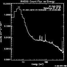
Here's an example in which we set all of the control parameters listed above and plot the spectrum (shown on right):
o=hsi_spectrum()
o -> set, obs_time_interval=['31-Oct-2010 01:12', '31-Oct-2010 01:24']
o -> set, sp_time_interval=2.
o -> set, sp_energy_binning=6
o -> set, seg_index_mask=[0, 0, 1, 1, 1, 0, 0, 0, 0, 0, 0, 0, 0, 0, 0, 0, 0, 0]
o -> set, /decimation_correct, /rear_decimation_correct
o -> plotman, sp_data_unit='Flux'
Energy and Time Binning
Energy Binning
There are a number of pre-defined binning schemes that set up the energy bins appropriately for different kinds of studies. Select one of the binning codes, e.g. code 11 for gamma-ray line flares,as follows:
o -> set, sp_energy_binning = 11
If you have a binning scheme that you think would be of general use, send your binning specifications to hessibugs@hesperia.nasa.gov, and we can add another binning code.
You can also define your own bins by specifying either a 1-D array of edges, or a 2-D array of start/end values, e.g.
o -> set, sp_energy_binning = [3.,4.,5.,8.,12., ...]
o -> set, sp_energy_binning = [[3.,4.], [4.,5.], ...]
o -> set, sp_energy_binning = 10.^(findgen(51)/52.*2.5) ; 50 logarithmically spaced bin from 1. to 253.
Time Binning
There are three control parameters that specify the time interval and binning:
- obs_time_interval - start/end of overall time interval in absolute time format
- time_range - normally [0.,0.] meaning use all of obs_time_interval. Or, can specify a start/end time in seconds relative to start of obs_time_interval to use. Or can specify an absolute interval, which will supercede obs_time_interval.
- sp_time_interval - If scalar, then this is width of bins in seconds. If an array, then defines the edges of the time bins, and must be in absolute time.
Note: Absolute time format means a fully referenced time in any ANYTIM format, e.g. '3-mar-05 12:36:44'. If you supply an absolute time as a number, it is interpreted as seconds since 1-jan-1979 00:00 (and should be double precision).
For example, to set up 2-second time bins for the period 31-Oct-2010 01:11:56 to 31-Oct-2010 01:23:28,
o -> set, obs_time_interval = ['31-Oct-2010 01:11:56.000', '31-Oct-2010 01:23:28.000']
o -> set, sp_time_interval = 2.
Retrieving Data, Livetime, and Time/Energy Bins
The sp_data_unit and sp_data_struct control parameters specify how the getdata method returns the spectrum data. The units of the data are specified by setting sp_data_unit to 'counts', 'rate', or 'flux' (default is 'counts'). Note that for rate, the units are per detector, i.e. counts sec-1 detector-1.
By default ,getdata returns an array dimensioned [nenergy,ntime]. If sp_data_struct is set to 1, then it returns an array of ntime structures containing the following tags
ut - [2], start/end of time bin in seconds since 1-Jan-1979
counts - [nenergy], counts in each energy bin
ecounts - [nenergy], error in counts in each energy bin
ltime - [nenergy], live time fraction in each energy bin
when the requested units are counts. The counts, ecounts tags become rate, erate for rate units, and flux, eflux for flux units. For example, if you have 173 time bins and 897 energy bins,
d = o-> getdata(sp_data_unit='flux', /sp_data_struct)
help,d
D STRUCT = -> <Anonymous> Array[173]
help,d,/st
** Structure <8d45c68>, 4 tags, length=10784, data length=10780, refs=1:
UT DOUBLE Array[2]
FLUX FLOAT Array[897]
EFLUX FLOAT Array[897]
LTIME FLOAT Array[897]
The time bins (also in the data structure, d.ut, above) and energy bins can be retrieved by calling getaxis. For example,
utbins = o -> getaxis(/ut)
ebins = o -> getaxis(/energy)
returns the midpoints of the time and energy bins. Use /mean, /gmean, /width, /edges_2, or /edges_1 in the getaxis call to return the arithmetic mean, geometric mean, width, 2xn edges, or 1-D edges.
So, for example, to plot the lowest energy bin of the flux as a time profile:
utplot, anytim(utbins, /ext), d.flux[0], /ylog, psym=10
or to plot the spectrum of the fifth time interval:
plot, ebins, d[5].flux, /xlog, /ylog, psym=10
Plotting Spectra, Time Profiles, and Spectrograms
After setting all of the desired parameters in the spectrum object, you can plot the data as a time profile, spectrum, or spectrogram using the plot (simple graphics window) or plotman (interactive plot manipulation widget) method. The livetime can also be plotted.
Here are some of the commonly used keywords for the plot and plotman methods:
- /pl_energy - plot spectrum (the default)
/pl_time - plot time profile
/pl_spec - plot spectrogram
/pl_ltime_used - plot livetime used (includes decimation and gaps)
/pl_ltime_ctr - plot corrected livetime counter - sp_data_unit - units for plot = 'counts', 'rate', 'flux'
- plotman_obj - plotman object reference to use, or if it doesn't exist yet, the plotman object that is created.
- /xlog, /ylog, /log_scale - plot log in x or y dimension, or for spectrogram
- legend_loc - 0/1/2/3/4/5/6 = no legend/ topleft/topright/ bottomleft/bottomright/outside left/ outside right
- /saa, /night, /flare, /decimation, /attenuator, /fast_rate - enables the indicators for those conditions on time plots
- dim1_color - array of colors to use
- dim1_sum - 0/1 = don't / do sum times (for spectrum plot) or energies (for time plot)
- dim1_use - time bins to use (for spectrum plot) or energy bins to use (for spectrum plot)
- Plus most IDL plot options like psym, charsize, thick, etc. (x, y, and main title can not be set by user though)
Examples:
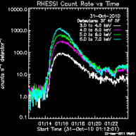
1. Time profile plot in plotman of the lowest four energy bins in rate units. Plotman panel named 'Time profile'.
o -> plotman, /pl_time, sp_data_unit='rate', /ylog, dim1_use=[0,1,2,3],dim1_sum=0, legend_loc=2, plotman_obj=p, desc='Time profile'
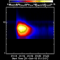
2. Spectrogram in flux units, log-scaled and smoothed, same plotman instance as Example 1. Plotman panel named 'Smoothed spectrogram'.
o -> plotman, /pl_spec, sp_data_unit='flux', /ylog, /log_scale, /interpolate, plotman_obj=p, desc='Smoothed spectrogram'
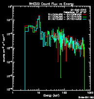
3. Spectrum plot of time intervals 2, 4, and 6 in simple graphics window with colors.
linecolors
ut = o->getaxis(/ut)
color = intarr(n_elements(ut))
use = [2,4,6]
color[use]=[2,7,9]
o -> plot, sp_data_unit='flux', dim1_sum=0, dim1_color=color, dim1_use=use
- Example 1.
- Example 2.
- Example 3.
Livetime, Gaps, Decimation, Attenuators
Livetime Counter
The livetime fraction for each spectrum time bin from the livetime counters for each of the 18 detector segments is available in an info parameter, livetime_ctr, e.g.
help, o->get(/livetime_ctr)
<Expression> FLOAT = Array[174, 18] ; 174 time bins, 18 segments
Livetime Used
However the livetime that is used to calculate the spectrum in rate or flux units includes the effect of data gaps, decimation, and any other mechanism that reduces the data counts. This 'used' livetime is available when you call getdata and request structure output, e.g.
data = o->getdata(/sp_data_struct)
help,data,/st
** Structure <5dcdd40>, 4 tags, length=944, data length=940, refs=1:
UT DOUBLE Array[2]
COUNTS FLOAT Array[77]
ECOUNTS FLOAT Array[77]
LTIME FLOAT Array[77]
data.ltime is dimensioned nenergy x ntime just to have the same dimensions as the counts and ecounts fields, but the values for each time bin are the same for all energies. Also, note that the values are not available for separate detectors.
Since the corrections for decimation and data gaps (and other effects?) are handled by adjusting the livetime, if you view the data in count space, the corrections are not in effect.
Decimation Correction
Front and rear detector decimation correction can be controlled separately via the decimation_correct and rear_decimation_correct control parameters. There are two info parameters you can examine for information about the decimation correction that was applied - decim_table and decim_warning.
As mentioned above the decimation correction is applied through changes in the livetime.
Attenuator Changes
Changes in attenuator state are not corrected for in the spectrum object. There are two options for generating a plot without the jumps caused by attenuator state changes:
- Use the heuristic corrections in the Observing Summary Data
- Import the spectrum and SRM data into OSPEX and determine the best-fit model.
For more information, see the FAQ question on this subject here.
Spectrum and SRM FITS Files
In order to perform spectral analysis, you must write a spectrum and response matrix (also called SRM or DRM) file from the spectrum object via the filewrite method.
To write the spectrum and full SRM files with auto-generated names, use this command:
spectrum_object-> filewrite, /buildsrm, all_simplify=0
The full list of keywords for the filewrite method are:
- buildsrm: 0/1 means don't / do write SRM file
- namedialog: 1 means provide widget for specifying names for output file(s)
- specfile: Name of spectrum FITS file
- srmfile: Name of SRM FITS file
- all_simplify: Specifies the type of SRM matrix to write
- 0: Full calculation of diagonal, off diagonal terms
- 1: Off diagonal terms are an approximation
- 2: Diagonal terms only
- 3: Diagonal terms only, and all = 1 (or zero if it's a normally off-diagonal matrix)
Unfortunately since information is combined when writing the files, these files can not be read back into the spectrum object. They can be used as input to OSPEX.
To write separate detector files with native energy bins (preserves the highest fidelity of the detector resolution), use the hsi_spectrum_sep_det_files routine (see header for calling arguments) or use the button in the Spectrum GUI.
If the spectrum time interval crosses attenuator state changes, the SRM file that is written will include the response matrix for each attenuator state encountered (and OSPEX will use the correct one during spectral analysis).
Semi Calibrated Option; Pileup Correction
The spectrum object has the option to produce semi-calibrated data, and to correct for pileup. Neither of these options is very accurate and we recommend not using them.
If you enable the SP_SEMI_CALIBRATED option, the diagonal response is used to compute an approximation of the photon spectrum, however no correction for grid variation, pileup, or background is done.
The pileup correction used in the spectrum object (enabled by setting PILEUP_CORRECT) does not ???. A better option is to disable the pileup correction in the spectrum object, but in further analysis in OSPEX, include the pileup_mod function component if you think there is pileup in the spectrum. In OSPEX, the pileup correction is more reliable because it is done in the forward direction, finding the values of pileup parameters that best approximate the photon model.
Processing Considerations
- 432 bytes are required per Time/Energy bin. Choose time resolution and energy binning with this constraint in mind.
- It is most efficient to process all energy bins needed for a given time range.
- To produce a spectrogram from 80 Mbyte of event data using a 1.7 GHz PC, allow 100 seconds.